Velten K. Mathematical Modeling and Simulation: Introduction for Scientists and Engineers

Подождите немного. Документ загружается.

4.3 Some Theory You Should Know 245

hyperbolic PDEs are (in this order):

+ u

+···=0 (4.38)

+ ...= 0 (4.39)

− u

+···=0 (4.40)

Referring to the standard form, one can, thus, say that elliptic PDEs are

characterized by the fact that they contain second-order derivatives with respect

to all independent variables, which all have the same sign when they are written

on one side of the equation. Parabolic PDEs involve one second-order derivative

and at least one ﬁrst-order derivative. Note that Deﬁnition 4.1 requires that there

must be at least one ﬁrst-order derivative in the ‘‘···’’ of Equation 4.39 (otherwise,

that equation would be an ODE). Finally, hyperbolic equations can be described

similar to elliptic equations except for the fact that the second-order derivatives

have opposite signs when brought on one side of the equation.

Comparing Equations 4.34 and 4.39, you see that the heat equation is an example

of a parabolic PDE. The stationary case of the two-dimensional heat equation (4.1)

is an example of an elliptic PDE. As was mentioned before, a stationary solution of

a PDE is a solution referring to the case where the time derivatives in the PDE

vanish. Solutions of this kind can usually be interpreted as expressing the state of

the system which is attained in a constant environment after a ‘‘very long’’ time

(mathematically, the state that is approached for t →∞). In this sense, stationary

solutions of the heat equation express the temperature distribution attained by a

system in a constant environment after a ‘‘very long’’ time. Using the index notation

for partial derivatives in Equation 4.1 and assuming T

= 0 in that equation, it turns

out that the two-dimensional stationary heat equation is

+ T

= 0 (4.41)

which corresponds to Equation 4.38, so we see that the stationary heat equation is

elliptic. Hyperbolic equations (Equation 4.40) are used to describe all kinds of wave

phenomena such as sound waves, light waves, or water waves [142].

Using appropriate methods of matrix algebra, the above classiﬁcation of PDEs

into elliptic, parabolic, and hyperbolic PDEs can be generalized to multidimensions

(i.e. PDEs depending on x

, ..., x

) [142]. This classiﬁcation is of particular impor-

tance in the numerical treatment of PDEs and will be discussed in Sections 4.6

and 4.8.

4.3.2

Initial and Boundary Conditions

Above we have seen that ODEs are usually solved by an entire family of solutions

unless initial or boundary conditions are imposed, which select one particular

solution among those many solutions (Section 3.7.1.1). For the same reason, initial

246 4 Mechanistic Models II: PDEs

or boundary conditions are used together with PDEs. From the mathematical

point of view, initial or boundary conditions are needed to make the mathematical

problem uniquely solvable. From the applications point of view, they are a necessary

part of the description of the system that is investigated. Considering Problem 1

in Section 4.1.3, for example, it is obvious from the applications point of view,

i.e. without any mathematical considerations, that this problem cannot be solved

unless we know the temperatures at the left and right ends of the cylinder (T

and T

) and the initial temperature distribution, T

(x). To solve Problem 1,wewill

use the one-dimensional form of the heat equation (4.33) (Section 4.6). Above we

have seen that this is a parabolic equation, and so we see here that this parabolic

equation requires a boundary condition referring to the spatial variable and an

initial condition referring to the time variable.

4.3.2.1 Well Posedness

Generally, the appropriate choice of initial and boundary conditions for PDEs can

be a subtle matter as discussed in [142]. It is related to the mathematical concept

of a well-posed problem, which was originally introduced by the French mathemati-

cian Hadamard. A well-posed differential equation problem satisﬁes the following

conditions [142]:

•

existence: a solution exists;

•

uniqueness: the solution is unique;

•

stability: the solution depends continuously on the data of the

problem.

Let us explain the last point referring to Problem 1 again. Assume a small change

in the temperature imposed at the left or right end of the cylinder, or small changes

in the initial temperature distribution. Then stability in the above sense means

that the change in the temperature distribution T(x, t) implied by your change

in the problem data should go to zero if you let the size of this change in the

data go to zero. This expresses our physical intuition, but you should know that

the discussion of stability matters and well-posedness matters in general can be

subtle (e.g. the appropriate deﬁnition of what is meant by ‘‘continuity’’). From a

mathematical point of view, we can thus say that initial or boundary conditions

have to be chosen in a way that makes the overall problem well posed in the above

sense.

4.3.2.2 A Rule of Thumb

The following ‘‘rule of thumb’’ for the proper selection of initial or boundary

conditions applies to many equations [138]:

Note 4.3.2 (Rule of thumb)

•

Elliptic equation: add a boundary condition

•

Parabolic equation: add a boundary condition for the space

variables and an initial condition at t = 0

4.3 Some Theory You Should Know 247

•

Hyperbolic equation: add a boundary condition and two initial

conditions at t = 0

Note that this is consistent with our above discussion of the initial and boundary

conditions of Problem 1, which was motivated by physical intuition. Generally, one

can say that physical intuition applied as above to Problem 1 frequently is a good

guideline for the proper choice of initial or boundary conditions.

Problem 2 from Section 4.1.3 gives us an example of boundary conditions for

an elliptic equation. In Section 4.9, this problem is solved using the stationary heat

equation. We have seen above that this is an elliptic equation in the two-dimensional

case (Section 4.3.1.3). Using appropriate methods of matrix algebra, the same can

be shown for the three-dimensional version of the stationary heat equation that is

used in the solution of Problem 2. Now looking at the formulation of Problem 2 in

Section 4.1.3, you see that this problem involves conditions for the space variables

at the boundary of the computational domain only, which is consistent with the

above ‘‘rule of thumb’’. Again, this is also consistent with physical intuition since

any change in the initial temperature distribution within the cube will certainly

affect the temperatures inside the cube for some time, but in the long run physical

intuition tells us that everything is determined by the constant conditions applied

at the boundaries of the cube and at its internal boundaries on the sphere surface

of Figure 4.1. For the hyperbolic case in the above ‘‘rule of thumb’’, appropriate

wave equation examples may be found in [138].

4.3.2.3 Dirichlet and Neumann Conditions

Note that two different kinds of boundary conditions are used in Problem 2.Onthe

top boundary of the cube and on the sphere surface, the value of the temperature is

prescribed. Boundary conditions that prescribe the values of the unknown function

of a PDE in this way are called Dirichlet boundary conditions. The remaining

boundaries of the cube are assumed to be ‘‘perfectly insulated’’ in Problem 2.

Perfect insulation means that there is no heat ﬂow across these boundaries. Using

vector notation, this can be expressed as follows: Let S denote one of the cube

boundaries, and let q(x)(Wm

−2

) be the heat ﬂow rate introduced in Section 4.2.

Then, if n(x) denotes the outward facing normal vector on S, q(x) ·n(x)(Wm

−2

)is

the (outward going) heat ﬂow through S, which is zero since S is insulated:

q(x) ·n(x) = 0 x ∈ S (4.42)

Using Fourier’s law (Equation 4.6), this turns into

∂T

∂n

=∇T · n(x) = 0 x ∈ S (4.43)

where ∂T/∂n denotes the normal derivative of T with respect to n, which expresses

T’s rate of change in the direction of n. Boundary conditions that prescribe the

248 4 Mechanistic Models II: PDEs

normal derivative of the unknown function such as Equation 4.43 are called

Neumann boundary conditions.Ifu is the unknown function in a PDE deﬁned on

adomain × I ⊂ R

× R and if S ⊂ ∂ is a subset of ’s boundary, the general

form of Dirichlet and Neumann boundary conditions in S can be written as [142]

Dirichlet: u(x, t) = f

(x, t)(x, t) ∈ S × I (4.44)

Neumann:

∂u(x, t)

∂n

= f

(x, t)(x, t) ∈ S × I (4.45)

where f

and f

are given real functions. Another frequently used boundary

condition is the Robin boundary condition, which speciﬁes a linear combination of

u and ∂u/∂n as follows:

Robin: a(x, t)u(x, t) +b(x, t)

∂u(x, t)

∂n

= f

(x, t)(x, t) ∈ S × I (4.46)

Any of the above three boundary conditions is called homogeneous if its right-hand

side vanishes (e.g. f

(x, t) = 0), otherwise inhomogeneous. A homogeneous Neu-

mann condition (f

(x, t) = 0inEquation4.45)isalsoknownasano-ﬂow condition.

Equation 4.43 is an example of such a homogeneous Neumann condition, which

forbids any heat ﬂow through S as discussed above. Similar interpretations apply

in many other situations, and this is why the term ‘‘no-ﬂow condition’’ is used.

Note that no-ﬂow conditions can sometimes also be interpreted as expressing the

symmetry of a problem, and hence the term symmetry boundary condition is also

used. An example of this along with further explanations is given in Section 4.3.3.

Regarding Problem 1 and Problem 2 in Section 4.1.3, the above discussion can be

summarized as follows:

•

Problem 1 imposes an initial condition in the domain

0 < x < 1 and two Dirichlet conditions at x = 0andx = 1.

The Dirichlet condition at x = 0(orx = 1) is

inhomogeneous if a nonzero temperature is imposed there,

homogeneous otherwise.

•

Problem 2 imposes Dirichlet conditions at the top surface of

thecubeandatthespheresurface(homogeneousor

inhomogeneous Dirichlet conditions depending on the

actual values of T

and T

), and a homogeneous Neumann

condition (no-ﬂow condition) at the remaining sides of the

cube.

4.3.3

Symmetry and Dimensionality

In practice, most PDEs cannot be solved in closed form, which means that they

are solved using numerical algorithms in most cases. The application of such

numerical algorithms can be extremely expensive in terms of computation time

and machine requirements such as memory or processor speed requirements [150].

4.3 Some Theory You Should Know 249

As has been already mentioned in Section 3.6.1, it may take several hours, days, or

even longer to solve complex coupled multidimensional PDE problems, even if you

are using supercomputers or large computer clusters (i.e. a great number of coupled

computers that work together to solve your problem). The continuous increase of

processor speeds and available memory does not change this situation since the

increase in computer power is accompanied by a similarly increasing complexity of

the problems that are solved. As faster computers become available, people begin

to solve problems that were beyond the scope of the old computer generation.

Therefore, the reduction of computation time and machine requirements is an

important issue in the solution of PDEs. As is explained below, a lot can be

achieved by the use of fast and efﬁcient numerical algorithms, by the intelligent

use of these algorithms, and by using appropriate fast and efﬁcient software.

But there is one thing you can do at an early stage before the application of

numerical algorithms: you can analyze the symmetry and dimensionality of your

problem.

Note 4.3.3 (Symmetry/dimensionality should be exploited) Based on a wise

consideration of symmetry and dimensionality, the complexity of a problem

and its computation time and machine requirements can often be substantially

reduced.

4.3.3.1 1D Example

To understand the point, consider the following Problem 3 (a modiﬁcation of

Problem 2 discussed in Section 4.1.3):

Problem 3:

Referring to the conﬁguration in Figure 4.4a and assuming

•

a constant temperature T

at the top surface of the cube (z = 1),

•

a constant temperature T

at the bottom surface of the cube

(z = 0),

•

and a perfect thermal insulation of all other surfaces of the cube,

what is the stationary temperature distribution T(x, y, z) within the cube?

It is simple to see that the solution of this problem will depend on z only, that

is, the resulting stationary temperature distribution will be of the form T(z)(see

the discussion of Problem 2 in Section 4.1.3 to understand what is meant by the

term ‘‘stationary temperature distribution’’). If there would be any temperature

differences in some given plane z = a inside the cube (0 ≤ a ≤ 1), then there

would be a point (x, y, a) in that plane where we would have either

∂T(x ,y,a)

∂x

= 0or

∂T(x ,y,a)

∂y

= 0. This would initiate a heat ﬂow according to Fourier’s law (Equation

4.6), which would then tend to ﬂatten out the temperature gradient at that point

until

∂T(x ,y,a)

∂x

∂T(x ,y,a)

∂y

= 0 would be achieved in the stationary limit. Similar to the

250 4 Mechanistic Models II: PDEs

0.8

0.6

0.4

0.2

0.8

0.6

0.4

0.2

(

)(

)

0.8

0.6

0.4

0.2

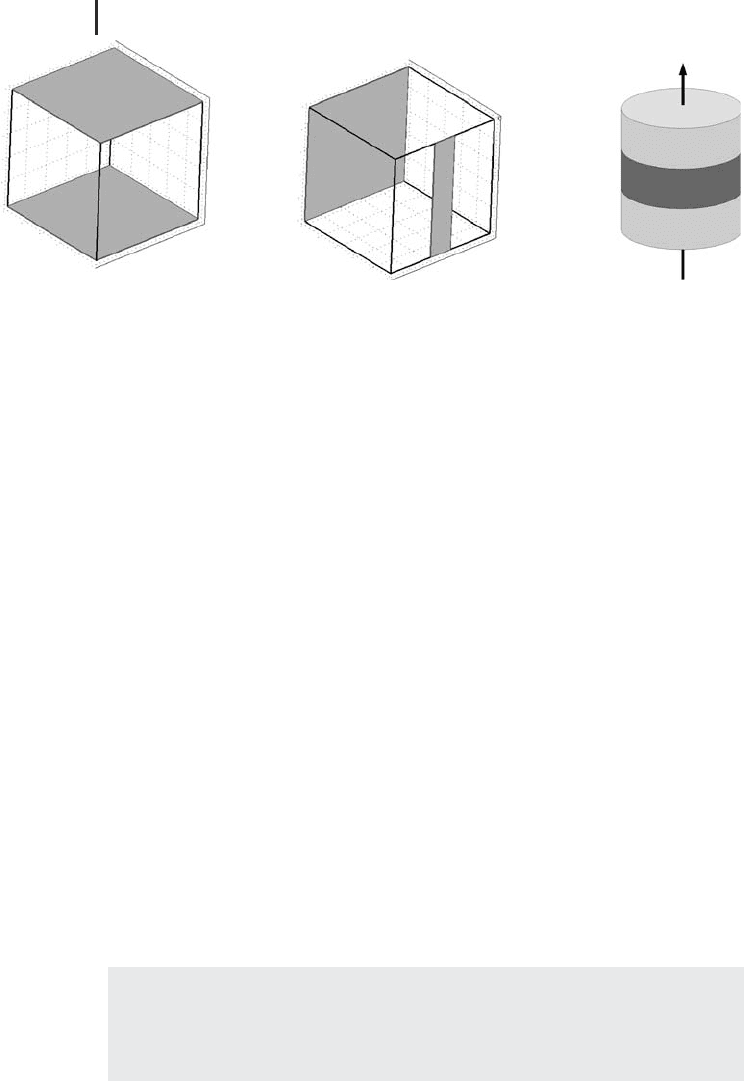
Fig. 4.4 (a) Cube [0, 1]

with highlighted boundaries z = 0

(bottom surface) and z = 1(topsurface)usedinProblem 3.

(b) Cube [0, 1]

with highlighted boundaries y = 1(backsur-

face) and y = 0, 0.4 ≤ x ≤ 0.6 (strip on the front surface)

used in Problem 4. (c) Cylinder used in Problem 5.

derivation of Equation 3.70 in Section 3.5.5, the stationary temperature distribution

that solves Problem 3 can be derived from the heat equation as follows:

T(x, y, z) = T

+ (T

− T

) · z (4.47)

Since T(x, y, z) depends on z only, this can also be written as

T(z) = T

+ (T

− T

) · z (4.48)

Such a temperature distribution that depends on one space coordinate only is

called a one-dimensional temperature distribution, and the corresponding physical

problemfromwhichitisderived(Problem 4 in this case) is called a one-dimensional

problem. Correspondingly, the solution of a two-dimensional (three-dimensional)

problem depends on two (three) space coordinates. Intuitively, it is clear that

it is much less effort to compute a one-dimensional temperature distribution

T(x) compared to higher dimensional distributions such as T(x, y)orT(x, y, z).

The discussion of the PDE solving numerical algorithms in Section 4.5 indeed

shows that the number of unknowns in the resulting systems of equations –

and hence the overall computational effort – depends dramatically on the

dimension.

Note 4.3.4 (Dimension of a PDE problem) The solution of one-dimensional

(two-dimensional, three-dimensional) PDE problems depends on one (two, three)

independent variables. To reduce the computational effort, PDEs should always

be solved using the lowest possible dimension.

4.3 Some Theory You Should Know 251

4.3.3.2 2D Example

Consider the following problem:

Problem 4:

Referring to the conﬁguration in Figure 4.4b and assuming

•

a constant temperature T

at the back surface of the cube (y = 1),

•

a constant temperature T

at the strip y = 0, 0.4 ≤ x ≤ 0.6atthe

front surface of the cube,

•

and a perfect thermal insulation of all other surfaces of the cube,

what is the stationary temperature distribution T(x, y, z) within the cube?

In this case, it is obvious that the stationary temperature distribution will depend

on x and y. Assuming T

> T

, for example, it is clear that the stationary temperature

will go down toward T

as we move in the y direction toward the (colder) back

surface, and it is likewise clear that the stationary temperature will increase as we

move in the x direction toward x = 0.5, the point on the x axis closest to the (warm)

strip on the front surface (see also the discussion of Figure 4.5b further below).

On the other hand, there will be no gradients of the stationary temperature in the

z direction. To see this, a similar ‘‘ﬂattening out’’ argument could be used as in

our above discussion of Problem 3. Alternatively, you could observe that the same

stationary temperature distribution would be obtained if the cube would extend

inﬁnitely in the positive and negative z direction, which expresses the symmetry

0 0.4 0.5 0.6

0.4 0.5 0.6

(b)(a)

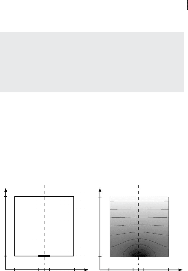
Fig. 4.5 Example of a reduction of the computational do-

main due to symmetry: (a) Geometry. (b) Solution of

Problem 4forT

= 20

◦

CandT

= 0

◦

C (computed using

Salome-Meca). Colors range from white (20

◦

C) to black

◦

C), lines in the domain are temperature isolines.

252 4 Mechanistic Models II: PDEs

of this problem in the z direction. More precisely, this expresses the translational

symmetry of this problem in the z direction, as you could translate the cube of

Problem 4 along the ‘‘inﬁnitely extended cube’’ arbitrarily in the z direction without

changing the stationary temperature distribution. This and other kinds of spatial

symmetries can often be used to reduce the spatial dimensionality of a problem,

and hence to reduce the computation time and machine requirements of a PDE

problem [151].

4.3.3.3 3D Example

Problem 2 in Section 4.1.3 is an example of a three-dimensional problem. In this

case, there are no symmetries that could be used to reduce the spatial dimensionality

of the problem. The stationary temperature in any particular point (x, y, z) depends

in a complex three-dimensional manner on the point’s relative position toward

thesphereandthetopsideofthecubeinFigure4.1b.Thereis,however,akind

of symmetry in Problem 2 that can at least be used to reduce the computational

effort (although the problem remains three dimensional). Indeed, it is sufﬁcient

to compute the temperature distribution in a quarter of the cube of Figure 4.1b,

which corresponds to (x, y) ∈ (0, 0.5) × (0, 0.5). The temperature distribution in

this quarter of the cube can then be extended to the other three quarters using the

mirror symmetry of the temperature distribution inside the cube with respect to the

planes y = 0.5andx = 0.5. See the discussion of Figure 4.5 for another example

of a mirror symmetry.

In the discussion of the ﬁnite-element method (Section 4.7), it will become clear

that the number of unknowns is reduced by about 75% if the computational domain

is reduced to a quarter of the original domain, so you see that the computational

effort is substantially reduced if Problem 2 is solved using the mirror symmetry.

However, note that we will not use the mirror symmetry when Problem 2 is solved

using Salome-Meca in Section 4.9, simply because the computational effort for this

problemisnegligibleevenwithoutthemirrorsymmetry(andwesavetheeffort

that would be necessary to extend the solution from the quarter of the cube into

the whole cube in the postprocessing step, see Section 4.9.4).

4.3.3.4 Rotational Symmetry

As another example of how the spatial dimension of a problem can be reduced due

to symmetry, consider

Problem 5:

Referring to the conﬁguration in Figure 4.4c and assuming

•

a constant temperature T

at the top surface of the cylinder,

•

a constant temperature T

at the dark strip around the cylinder,

•

and a perfect thermal insulation of all other surfaces of the

cylinder,

what is the stationary temperature distribution T(x, y, z) within the cylinder?

4.3 Some Theory You Should Know 253

In this case, it is obvious that the problem exhibits rotational symmetry in

the sense that the stationary temperature distribution is identical in any vertical

section through the cylinder that includes the z axis (a reasoning similar to

the ‘‘ﬂattening out’’ argument used in Section 4.3.3.1 would apply to temperature

distributions deviating from this pattern). Using cylindrical coordinates (r, φ, z), this

means that we will get identical stationary temperature distributions on any plane

φ = const. Hence, the stationary temperature distribution depends on the two

spatial coordinates r and z only, and Problem 5, thus, is a two-dimensional problem.

Note that in order to solve this problem in two dimensions, the heat equation

must be expressed in cylindrical coordinates (in particular, it is important to

choose the appropriate model involving cylindrical coordinates if you are using

software).

4.3.3.5 Mirror Symmetry

Consider Figure 4.5a, which shows the geometrical conﬁguration of the two-

dimensional problem corresponding to Problem 4. AsinProblem 4, we assume

a constant temperature T

for y = 1 (the top end of the square in Figure 4.5a),

a constant temperature T

in the strip y = 0, 0.4 ≤ x ≤ 0.6 (the thick line at the

bottom end of the square in Figure 4.5a), and a perfect thermal insulation at all

other boundary lines of the square. Again, we ask for the stationary temperature

within the square. As discussed above, the solution of this problem will then

also solve Problem 4 due to the translational symmetry of Problem 4 in the z

direction.

Note that the situation in Figure 4.5a is mirror symmetric with respect to

the dashed line in the ﬁgure (similar to the mirror symmetry discussed in

Section 4.3.3.3). The boundary conditions imposed on each of the two sides of the

dashed line are mirror symmetric with respect to that line, and hence the resulting

stationary temperature distribution is also mirror symmetric with respect to that

dashed line. This can be seen in Figure 4.5b, which shows the solution of Problem 4

computed using Salome-Meca (Section 4.9). So we see here that it is sufﬁcient to

compute the solution of Problem 4 in one half of the square only, for example, for

x < 0.5, and then to extend the solution into the other half of the square using

mirror symmetry. In this way, the size of the computational domain is reduced

by one half. This reduces the number of unknowns by about 50% and leads to

a substantial reduction of the computational effort necessary to solve the PDE

problem (see Section 4.5 for details).

4.3.3.6 Symmetry and Periodic Boundary Conditions

In all problems considered above, we have used ‘‘thermal insulation’’ as a boundary

condition. As discussed in Section 4.3.2.3 above, this boundary condition is

classiﬁed as a Neumann boundary condition, and it is also called a no-ﬂow

condition since it forbids any heat ﬂow across the boundary. Referring to Problem 4

and Figure 4.4b, the thermal insulation condition serves as a ‘‘no-ﬂow’’ condition

in this sense, for example, at the cube’s side surfaces x = 0andx = 1andatthe

254 4 Mechanistic Models II: PDEs

cube’s front surface besides the strip. At the top and bottom surfaces of the cube,

the thermal insulation condition can be interpreted in the same way, but it can also

be interpreted there as expressing the symmetry of the problem in the z direction.

As was explained in Section 4.3.3.2, Problem 4 can be interpreted as describing

a situation where the cube extends inﬁnitely into the positive and negative z

directions. In this case, the ‘‘no-ﬂow’’ condition at the top and bottom surfaces of

the cube in Figure 4.4b would not be a consequence of a thermal insulation at

these surface – rather, it would be a consequence of the symmetry of the problem

which implies that there can be no temperature gradients in the z direction. This is

why no-ﬂow conditions are often also referred to as symmetry boundary conditions.

Finally, we remark that substantial reductions of the complexity of a PDE problem

can also be achieved in the case of periodic media. For periodic media such as the

medium shown in Figure 4.3, it will usually be sufﬁcient to compute the solution

of a PDE on a single periodicity cell along with appropriate periodic boundary

conditions at the boundaries of the periodicity cell. An example of this and some

further explanations is given in Section 4.10.2.1.

4.4

Closed Form Solutions

InSection3.6,wehaveseenthatODEscanbesolvedeitherinclosedformor

numerically. As was discussed there, closed form solutions can be expressed in

terms of well-known functions such as the exponential function and the sine

function, while the numerical approach is based on the approximate solution of

the equations on the computer. All these hold for PDEs as well, including the fact

that closed form solutions cannot be obtained in most cases – they are like ‘‘dust

particles in the ODE/PDE universe’’ as discussed in Section 3.7.4. Since PDEs

involve derivatives with respect to several variables and, thus, can express a much

more complex dynamical behavior compared to ODEs, it is not surprising that

one can generally say that it is even harder to ﬁnd closed form solutions of PDEs

compared to ODEs.

Nevertheless, as was explained in Section 3.6, it is always a good idea to look

for closed form solutions of differential equations since they may provide valuable

information about the dependence of the solution on the parameters of the system

under investigation. A great number of techniques to derive closed form solutions

of differential equations – PDEs as well as ODEs – has been developed, but an

exhaustive treatment of this topic is beyond the scope of a ﬁrst introduction

into mathematical modeling. Since closed form solutions are unavailable in most

cases, we will conﬁne ourselves here to an example derivation of a closed form

solution for the one-dimensional heat equation. Readers who want to know more

on closed form solution techniques are referred to appropriate literature such

as [152].