Velten K. Mathematical Modeling and Simulation: Introduction for Scientists and Engineers

Подождите немного. Документ загружается.

4.4 Closed Form Solutions 255

4.4.1

Problem 1

So let us reconsider the one-dimensional heat equation now (Equation 4.1 in

Section 4.2):

∂T

∂t

Cρ

∂

∂x

(4.49)

As discussed in Section 4.3.2, this equation needs boundary conditions for the

space variables and an initial condition at t = 0. Assuming (0, L)asthespatial

domain in which Equation 4.49 is solved (that is, x ∈ (0, L)), let us consider the

following initial and boundary conditions:

T(0, t) = 0 ∀t ≥ 0 (4.50)

T(L, t) = 0 ∀t ≥ 0 (4.51)

T(x,0)= T

∀x ∈ (0, L) (4.52)

where T

∈ R is a constant initial temperature. Note that this corresponds to Problem

1 in Section 4.1.3 with T

(x) = T

and T

= T

= 0. As was explained there, you can

imagine, for example, a cylindrical body as in Figure 4.1a with an initial, constant

temperature T

, the ends of this body being in contact with ice water after t = 0.

4.4.2

Separation of Variables

The above problem can now be solved using a separation of variables tech-

nique [111]. Note that a similar technique has been described for ODEs in Section

3.7.2. This method assumes a solution of the form

T(x, t) = a(x) · b(t) (4.53)

where the variables x and t involve separate functions a and b. Substituting Equation

4.53 in Equation 4.49 you get

db(t)/dt

Cρ

· b(t)

a(x)/dx

a(x)

(4.54)

Both sides of the last equation must equal some constant −k

with k = 0(itcan

be shown that T would be identically zero otherwise). This leads to a system of two

uncoupled ODEs:

db(t)

+ k

Cρ

b(t) = 0 (4.55)

256 4 Mechanistic Models II: PDEs

a(x)

+ k

a(x) = 0 (4.56)

Equation 4.55 can be solved using the methods in Section 3.7, which leads to

b(t) = Ae

−k

K/Cρt

(4.57)

where A is some real constant. The general solution of Equation 4.56 is

a(x) = B

· sin(kx) + B

· cos(kx ) (4.58)

where B

and B

are real constants. Equation 4.50 implies

= 0 (4.59)

and Equation 4.51 gives

kL = nπ (4.60)

k = k

nπ

(4.61)

for some n ∈ N.Thusforanyn ∈ N, we get a solution of Equation 4.56:

a(t) = B

· sin(k

x ) (4.62)

Using Equations 4.53, 4.57, and 4.62 gives a particular solution of Equations

4.49–4.51 for any n ∈ N as follows:

(x, t) = A

· sin(k

x ) · e

−k

Cρ

(4.63)

Here, A

is a real constant. The general solution of Equations 4.49–4.51 is then

obtained as a superposition of the particular solutions in Equation 4.63:

T(x, t) =

∞



n=1

(x, t) =

∞



n=1

· sin(k

x ) · e

−k

Cρ

(4.64)

The coefﬁcients A

in the last equation must then be determined in a way such

that the initial condition in Equation 4.52 is satisﬁed:

= T(x,0)=

∞



n=1

· sin(k

x ) (4.65)

This can be solved for the A

using Fourier analysis as described in [111], which

ﬁnally gives the solution of Equations 4.49–4.52 as follows:

T(x, t) =

∞



n=1,3,5,...

nπ

· sin(k

x ) · e

−k

Cρ

(4.66)

4.5 Numerical Solution of PDE’s 257

The practical use of this expression is, of course, limited since it involves an

inﬁnite sum, which can only be evaluated approximately. An expression such as

Equation 4.66 is at what might be called the borderline between closed from solutions

and numerical solutions, which will be discussed in the subsequent sections. The

fact that we are getting an inﬁnite series solution for a problem such as Equations

4.49–4.52 – which certainly is among the most elementary problems imaginable

for the heat equation – conﬁrms our statement that numerical solutions are even

more important in the case of PDEs compared to ODEs.

4.4.3

A Particular Solution for Validation

Still, closed form solutions are of great use, for example, as a test of the correctness

of the numerical procedures. Remember that a comparison with closed form

solutions of ODEs was used in Section 3.8 to demonstrate the correctness of the

numerical procedures that were discussed there (e.g. Figure 3.9 in Section 3.8.2).

Inthesameway,wewillusetheparticularsolutionT

(x, t)fromEquation4.63as

a means to validate the ﬁnite difference method that is described in Section 4.6.

Assuming A

= 1inEquation4.63,T

turns into

∗

(x, t) = sin





· e

−

Cρ

(4.67)

which is the closed form solution of the following problem:

∂T

∂t

Cρ

∂

∂x

(4.68)

T(0, t) = 0 ∀t ≥ 0 (4.69)

T(L, t) = 0 ∀t ≥ 0 (4.70)

T(x,0)= T

∗

(x,0)= sin





∀x ∈ (0, L) (4.71)

4.5

Numerical Solution of PDE’s

Remember the discussion of the Euler method in Section 3.8.1.1. There, we wanted

to solve an initial-value problem for a general ODE of the form



(x) = F(x, y(x)) (4.72)

y(0) = a (4.73)

Analyzing the formulas discussed in Section 3.8.1, you will ﬁnd that the main idea

used in the Euler method is the approximation of the derivative in Equation 4.72

258 4 Mechanistic Models II: PDEs

bythedifferenceexpression



(x) ≈

y(x + h) − y(x)

(4.74)

Using similar difference expressions to approximate the derivatives, the same

idea can be used to solve PDEs, and this leads to a class of numerical methods

called ﬁnite difference methods (often abbreviated as FD methods) [140]. An example

application of the FD method to the one-dimensional heat equation is given in

Section 4.6. The application of the FD method is often the easiest and most natural

thing to do in situations where the computational domain is geometrically simple,

for example, where you solve an equation on a rectangle (such as the domain

[0, L] × [0, T] used in Section 4.6).

If the computational domain is geometrically complex, however, the formulation

of FD methods can be difﬁcult or even impossible since FD methods always need

regular computational grids to be mapped onto the computational domain. In such

situations, it is better to apply e.g. the ﬁnite-element method (often abbreviated as the

FE method ) described in Section 4.7. In the FE method, the computational domain

is covered by a grid of approximation points that do not need to be arranged in a

regular way as it is required by the FD method. These grids are often made up of

triangles or tetrahedra, and it is seen later that they can be used to describe even

very complex geometries.

Similar to the numerical methods solving ODEs discussed in Section 3.8.1,

numerical methods for PDEs are discretization methods in the sense that they

provide a discrete reformulation of the original, continuous PDE problem. While

the discussion in this book will be conﬁned to FD and FE methods, you should

note that there is a number of other discretization approaches, most of them

speciﬁcally designed for certain classes of PDEs. For example, PDEs that are

formulated as an initial-value problem in one of its variables can be treated by the

method of lines, which basically amounts to a reformulation of the PDE in terms of

a system of ODEs or differential-algebraic equations [153]. Spectral methods are a

variant of the FE method involving nonlocal basis functions such as sinusoids or

Chebyshev polynomials, and they work best for PDEs having very smooth solutions

as described in [154]. Finite volume methods are often applied to PDEs based on

conservation laws, particularly in the ﬁeld of CFD [155, 156].

4.6

The Finite Difference Method

4.6.1

Replacing Derivatives with Finite Differences

The FD method will be introduced now referring to the one-dimensional heat

equation 4.49 (see Section 4.2):

∂T

∂t

Cρ

∂

∂x

(4.75)

4.6 The Finite Difference Method 259

As was already mentioned above, the idea of the FD method is similar to

the idea of the Euler method described in Section 3.8.1.1: a replacement of the

derivatives in the PDE by appropriate difference expression. In Equation 4.75, you

see that we need numerical approximations of a ﬁrst-order time derivative and of a

second-order space derivative. Similar to the above derivation of the Euler method,

the time derivative can be approximated as

∂T(x, t)

∂t

≈

T(x, t + t) − T(x, t)

t

(4.76)

if t is a sufﬁciently small time step (which corresponds to the stepsize h of the

Euler method). To derive an approximation of the second-order space derivative,

let x be a sufﬁciently small space step. Then, second-order Taylor expansions of

T(x, t)give

T(x + x, t) = T(x, t) +

∂T(x, t)

∂x

x +

∂

T(x, t)

∂x

(

x

)

+··· (4.77)

T(x − x, t) = T(x, t) −

∂T(x, t)

∂x

x +

∂

T(x, t)

∂x

(

x

)

−··· (4.78)

Adding these two equations, a so-called central difference approximation of the

second-order space derivative is obtained:

T(x, t + t) − T(x, t)

t

≈

T(x + x, t) +T(x − x, t) − 2T(x, t)

(

x

)

(4.79)

The right-hand sides of Equations 4.76 and 4.79 are called ﬁnite difference approxi-

mations of the derivatives. As discussed in [157], a great number of ﬁnite difference

approximations can be used for any particular equation. An important criterion

for the selection of ﬁnite difference approximations is their order of accuracy.For

example, it can be shown that the approximation in Equation 4.79 is fourth order

accurate in x, which means that the difference between the left- and right-hand

side in Equation 4.79 can be expressed as c

(

x

)

+ c

(

x

)

···where c

, c

, ...

are constants [157]. Hence, the approximation error made in Equation 4.79 de-

creases quickly as x → 0. Note that the high accuracy of this approximation

is related to the fact that all odd terms cancel out when we add the two Taylor

expansions (4.77) and (4.78). Substituting Equations 4.76 and 4.79 in Equation 4.75

gives

T(x, t + t) − T(x, t)

t

≈

Cρ

T(x + x, t) + T(x − x, t) − 2T(x, t)

(

x

)

(4.80)

4.6.2

Formulating an Algorithm

Assume now we want to solve Equation 4.75 for t ∈ (0, T]andx ∈ (0, L)where

T = N

· t (4.81)

L = N

· x (4.82)

260 4 Mechanistic Models II: PDEs

for N

, N

∈ N. Let us deﬁne

= i · x, i = 0, ..., N

(4.83)

= j · t, j = 0, ..., N

(4.84)

i,j

= T(x

, t

), i = 0, ..., N

, j = 0, ..., N

(4.85)

Then, Equation 4.80 suggests the following approximation for i = 1, ..., N

− 1

and j = 0, ..., N

− 1:

i,j+1

= T

i,j

+ η



i+1,j

+ T

i−1,j

− 2T

i,j



(4.86)

where

η =

Kt

Cρx

(4.87)

We will now use Equation 4.86 to solve Equations 4.68–4.71, since the closed

form solution of these equations is the known expression T

∗

(x, t) in Equation 4.67,

which can then be used to assess the accuracy of the numerical procedure. Using

the notation of this section, Equations 4.69–4.71 can be written as follows:

0,j

= 0, j = 0, ..., N

(4.88)

= 0, j = 0, ..., N

(4.89)

i,0

= sin



ix



, i = 0, ..., N

(4.90)

Let us now write down Equation 4.86 for j = 0:

i,1

= T

i,0

+ η



i+1,0

+ T

i−1,0

− 2T

i,0



(4.91)

On the right-hand side of the last equation, everything is known from the initial

condition, Equation 4.90. Hence, Equation 4.91 can be used to compute T

i,1

for

i = 1, ..., N

− 1 (note that T

0,1

and T

are known from Equations 4.88 and

4.89). Then, all T

i,j

with j = 0orj = 1 are known and we can proceed with Equation

4.86 for j = 1:

i,2

= T

i,1

+ η



i+1,1

+ T

i−1,1

− 2T

i,1



(4.92)

Again, everything on the right-hand side is known, so we get T

i,2

for i =

1, ..., N

− 1 from the last equation. Proceeding in this way for j = 2, 3, ...,allT

i,j

for i = 0, ..., N

and j = 0, ..., N

are obtained successively.

4.6.3

Implementation in R

Obviously, the procedure just described consists of the application of two nested

iterations, or, in the language of programming languages: it consists of two nested

4.6 The Finite Difference Method 261

loops. The ﬁrst (outer) loop advances j from 0 to N

− 1, and within this loop there is

a second loop, which advances i from 1 to N

− 1. The entire algorithm is realized

in the R-program

HeatClos.r which is a part of the book software. The essential

part of this code consists of the two loops just mentioned:

1: for (j in 0:Nt){

2: for (i in 2:Nx)

3: T[i,2]=T[i,1]+eta*(T[i+1,1]+T[i-1,1]-2*T[i,1])

4: for (i in 2:Nx)

5: T[i,1]=T[i,2]

...

7: }

(4.93)

The outer loop over j is deﬁned in line 1 using Rs for command, which works

similar to Maximas

for command that was discussed in Section 3.8.1.2. This

commands iterates anything enclosed in brackets ‘‘

{...}’’ in lines 1–7, using

successive values

j = 0, j = 1, ...,j = Nt. The inner loop over i is in lines

2–3. The range of both the loops is slightly different from the ranges discussed

above for purely technical reasons (R does not allow arrays having index ‘‘0’’, and

hence all indices in

HeatClos.r begin with ‘‘1’’ instead of ‘‘0’’). The temperatures

are computed in line 3, which is in exact correspondence with Equation 4.86, except

for the fact that the index ‘‘2’’ is used here instead of ‘‘j + 1’’ and index ‘‘1’’ instead

of j. This means that

HeatClos.r stores the temperatures at two times only, the

‘‘new’’ temperatures in

T[i,2] and the ‘‘old’’ temperatures in T[i,1].Thisis

done to save memory since one usually wants to have the temperature at a few

times only as a result of the computation. In

HeatClos.r,avectorto deﬁnes these

fewpointsintimeandthe6ofthecode(whichwehaveleftouthereforbrevity).

After each time step, the next time step is prepared in lines 4–5 where the new

‘‘old’’ temperature is deﬁned as the old ‘‘new’’ temperature.

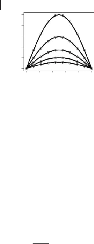
Figure 4.6 shows the result of the computation. Obviously, there is a perfect

coincidence between the numerical solution (lines) and the closed form solution,

Equation 4.67. As was mentioned above, you can imagine Figure 4.6 to express

the temperature distributions within a one-dimensional physical body such as the

cylinder shown in Figure 4.1a. At time 0, the top curve in the ﬁgure shows a

sinusoidal temperature distribution within that body, with temperatures close to

100

◦

C in the middle of that body and temperatures around 0

◦

Catitsends.The

ends of the body are kept at a constant temperature of 0

◦

C according to Equations

4.69 and 4.70. Physically, you can imagine the ends of that body to be in contact

with ice water. In such a situation, physical intuition tells us that a continuous heat

ﬂow will leave that body through its ends, accompanied by a continuous decrease

of the temperature within the body until T(x) = 0(x ∈ [0, 1]) is achieved. Exactly

this can be seen in the ﬁgure, and so you see that this solution of the heat equation

corresponds with our physical intuition. Note that the material parameters used

in this example (Figure 4.6 and

HeatClos.r) correspond to a body made up of

aluminum.

262 4 Mechanistic Models II: PDEs

100

0.0 0.2 0.4 0.6 0.8 1.0

Temperature (°C)

(

)

Fig. 4.6 Solution of Equations 4.68–4.71 for

K = 210 (cal/

◦

C/g), C = 900 (cal

◦

Cgs), ρ =

2700 (g/cm

), and L = 1. Lines: numerical

solution computed using

HeatClos.r based

on the ﬁnite difference scheme, Equation

4.86, at times t = 0, 625, 1250, 1875, 2500

s, which correspond to the lines from top

to bottom. Circles: closed form solution,

Equation 4.67.

4.6.4

Error and Stability Issues

In the general case, you will not have a closed form solution, which could be used as

in Figure 4.6 to assess the accuracy of the numerical solution. To control the error

within FD algorithms, you may look for error controlling algorithms that apply to

your speciﬁc FD scheme in the literature [3, 138, 150, 157]. Alternatively, you may

use the heuristic procedure described in Note 3.8.1, which means in this case that

you compute the solution ﬁrst using x and t, and then the second time using

x/2andt/2. As explained in Section 3.8.2.1, you may assume a sufﬁciently

precise result if the differences between these two solutions are negligibly small.

Any newly written FD program, however, should ﬁrst be checked using a closed

form solution similar to above.

Looking into

HeatClos.r, you will note that the time step t – which is denoted

Dt within HeatClos.r – is chosen depending on the space step x as follows:

t =

Cρx

(4.94)

If you increase t above this value, you will note that beyond a certain limit

the solution produced by

HeatClos.r becomes numerically unstable, that is, it

exhibits wild unphysical oscillations similar to those that we have seen in the

discussion of stiff ODEs in Section 3.8.1.4. The stability of the solution, hence, is

an issue for all kinds of differential equation including PDEs. If you apply ﬁnite

difference schemes such as Equation 4.86, you should always consult appropriate

literature such as [140] to make sure that your computations are performed within

the stability limits of the particular method you are using. In the case of the FD

scheme Equation 4.86, a von Neumann stability analysis shows that stability requires

4.6 The Finite Difference Method 263

η =

Kt

Cρx

(4.95)

to be satisﬁed [111]. This criterion is satisﬁed by choosing t according to

Equation 4.94 in

HeatClos.r.

4.6.5

Explicit and Implicit Schemes

The FD scheme Equation 4.86 is also known as the leap frog scheme since it

advances the solution successively from time level j = 1toj = 2, 3, ..., similar to

the children’s game leapfrog [111]. Since the solution at a new time level j + 1can

be computed explicitly based on the given right-hand side of Equation 4.86, this

FD scheme is called an explicit FD method.

An implicit variant of the FD scheme Equation 4.86 is obtained if Equation 4.80

is replaced by

T(x, t + t) − T(x, t)

t

≈

Cρ

T(x + x, t + t) +T(x − x, t + t) − 2T(x, t + t)

(

x

)

(4.96)

which leads to the approximation

i,j+1

− T

i,j

t

Cρ

i+1,j+1

+ T

i−1,j+1

− 2T

i,j+1

x

(4.97)

for i = 1, ..., N

− 1andj = 0, ..., N

− 1. The last equation cannot be solved for

i,j+1

as before. T

i,j+1

is expressed implicitly here since the equation depends on

other unknown temperatures at the time level j + 1: T

i+1,j+1

and T

i−1,j+1

.Given

some time level j, this means that the equations (4.97) for i = 1, ..., N

− 1are

coupled and must be solved as a system of linear equations. Methods of this

kind are called implicit FD methods. Implicit FD methods are usually more stable

compared to explicit methods at the expense of higher computation time and

memory requirements (since a system of linear equations must be solved in

any time step for the implicit scheme Equation 4.97, while the temperatures in

the new time step could be obtained directly from the explicit scheme Equation

4.86). The implicit method Equation 4.97, for example, can be shown to be

unconditionally stable, which means that no condition such as Equation 4.95 must

be observed to ensure stable results without those unphysical oscillations discussed

above [140].

TheFDmethodEquation4.86isalsoknownastheFTCS method [158]. To

understand this, consider Equation 4.80 on which Equation 4.86 is based: as

was mentioned above, the right-hand side of Equation 4.80 is a central difference

264 4 Mechanistic Models II: PDEs

approximation of the second space derivative, which gives the letters ‘‘CS’’ (Central

difference approximation in Space) of ‘‘FTCS’’. The left-hand side of Equation 4.80,

on the other hand, refers to the time level t used for the approximation of the

space derivative and to the time level t + t, that is, to a time level in the forward

direction. This gives the letters ‘‘FT’’ (Forward difference approximation in Time)

of ‘‘FTCS’’. The implicit scheme (Equation 4.97) can be described in a similar way,

except for the fact that in this case the approximation of the time derivative goes

into the backward direction, and this is why Equation 4.97 is also known as the

BTCS method.

Note that there is a great number of other FD methods beyond the methods

discussed so far, most of them speciﬁcally tailored for special types of PDEs [138,

150, 157, 158].

4.6.6

Computing Electrostatic Potentials

After solving the heat equation, let us consider a problem from classical electrody-

namics: the computation of a two-dimensional electrostatic potential U(x, y)based

on a given distribution of electrical charges, ρ(x, y). The electrostatic potential is

known to satisfy the following PDE [111]:

∂

U(x , y)

∂x

∂

U(x , y)

∂y

=−4πρ(x, y) (4.98)

According to the classiﬁcation in Section 4.3.1.3, this is an elliptic PDE which is

known as Poisson’s equation. Assume we want to solve Equation 4.98 on a square

(0, L) × (0, L). To formulate an FD equation, let us assume the same small space

step  = L/N in the x and y directions (N ∈ N). Then, denoting U

i,j

= U(i, j),

i,j

= ρ(i, j) and using the central difference approximation for the derivatives

similar as above, the following FD equation is obtained for i = 1, ..., N − 1and

j = 1, ..., N − 1:

i,j



i+1,j

+ U

i−1,j

+ U

i,j+1

+ U

i,j−1



+ πρ

i,j



(4.99)

Note that all U terms in this equation are unknown, and hence this is again a

coupled system of linear equations, similar to the implicit BTCS scheme discussed

above. Equations of this kind are best solved using the iterative methods that are

explained in the next section.

4.6.7

Iterative Methods for the Linear Equations

Systems of coupled linear equations such as Equation 4.99 arise quite generally

in the numerical treatment of PDEs, regardless of whether you are using FD

methods, FE methods (Section 4.7), or any of the other methods mentioned in