Versteeg H., Malalasekra W. An Introduction to Computational Fluid Dynamics: The Finite Volume Method

Подождите немного. Документ загружается.

3.7 RANS EQUATIONS AND TURBULENCE MODELS 97

effect for interactions between Reynolds stress production and streamline

curvature. They also included:

• Variable C

with a functional dependence on local strain rate S

and

vorticity Ω

• Ad hoc modiﬁcation of the

-equation to reduce the overprediction of

the length scale, leading to poor shear stress predictions in separated

ﬂows

• Wall-damping functions to enable integration of the k- and

-equation

to the wall through the viscous sub-layer

Leschziner (in Peyret and Krause, 2000) compared the performance of

linear and cubic k–

models with the RSM to demonstrates the performance

enhancement for an aerofoil computation at an incidence angle where trail-

ing edge separation has just occurred. The linear k–

model fails to indicate

the stall condition and gives poor accuracy for a range of other boundary

layer parameters, whereas the results of the cubic k–

model are very close to

those of the RSM.

3.7.5 Closing remarks --- RANS turbulence models

The ﬁeld of turbulence modelling provides an area of intense research

activity for the CFD and ﬂuid engineering communities. In the previous

sections we have outlined the modelling strategy of the most prominent

RANS turbulence models that are applied in or under development for

commercially available general-purpose codes. Behind much of the research

effort in advanced turbulence modelling lies the belief that, irrespective

of boundary conditions and geometry, there exists a (limited) number of

universal features of turbulence, which, when identiﬁed correctly, can form

the basis of a complete description of ﬂow variables of interest to an engineer.

The emphasis must be on the word ‘belief ’, because the very existence of

a classical model – based on time-averaged equations – of this kind is con-

tested by a number of renowned experts in the ﬁeld. Encouraged by, for

example, the early successes of the mixing length model in the external

aerodynamics ﬁeld, they favour the development of dedicated models for

limited classes of ﬂow. These two viewpoints naturally lead to two distinct

lines of research work:

1 Development and optimisation of turbulence models for limited

categories of ﬂows

2 The search for a comprehensive and completely general-purpose

turbulence model

Industry has many pressing ﬂow problems to solve that will not wait for the

conception of a universal turbulence model. The k–

model is still widely

used in industrial applications and produces useful results in spite of earlier

observations relating to its limited validity. Fortunately many sectors of

industry are speciﬁcally interested in a limited class of ﬂows only, e.g. pipe

ﬂows for the oil transportation sector, turbines and combustors for power

engineering. The large majority of turbulence research consists of case-

by-case examination and validation of existing turbulence models for such

speciﬁc problems.

ANIN_C03.qxd 29/12/2006 04:35PM Page 97

78 CHAPTER 3 TURBULENCE AND ITS MODELLING

stresses take over from turbulent Reynolds stresses at low Reynolds numbers

and in the viscous sub-layer adjacent to solid walls. The equations of the low

Reynolds number k–

model, which replace (3.44)–(3.46), are given below:

(3.51)

+ div(

kU) = div

+ grad k + 2

. S

−

ρε

(3.52)

+ div(

ρε

U) = div

+ grad

+ C

. S

− C

(3.53)

The most obvious modiﬁcation, which is universally made, is to include the

molecular viscosity

in the diffusion terms in (3.52)–(3.53). The constants

, C

and C

in the standard k–

model are multiplied by wall-damping

functions f

, f

and f

, respectively, which are themselves functions of the

turbulence Reynolds number (Re

=ϑ/

= k

εν

)), Re

= k

1/2

and/or

similar parameters. As an example we quote the Lam and Bremhorst (1981)

wall-damping functions:

= [1 − exp(−0.0165 Re

)]

1 +

= 1 +

= 1 − exp(−Re

) (3.54)

Equations (3.51)–(3.53) and the RANS equations need to be integrated to

the wall, but the boundary condition for

gives rise to problems. The best

available measurements suggest that the rate of dissipation of turbulent

energy rises steeply as the wall is approached and tends to an (unknown) con-

stant value. Lam and Bremhorst use

∂ε

∂

y = 0 as the boundary condition.

Other low Reynolds number k–

models are based on a modiﬁed dissipation

rate variable deﬁned as 6 =

− 2

(

∂

, introduced by Launder and

Sharma (1974), which allows us to use the more straightforward boundary

condition 6 = 0. It should be noted that the resulting equation set is numer-

ically stiff and the further appearance of non-linear wall-damping functions

regularly gives rise to severe challenges to achieve convergence.

Assessment of performance

The k–

model is the most widely used and validated turbulence model.

It has achieved notable successes in calculating a wide variety of thin shear

layer and recirculating ﬂows without the need for case-by-case adjustment of

0.05

20.5

∂

(

ρε

)

∂

(

∂

ANIN_C03.qxd 29/12/2006 04:34PM Page 78

3.7 RANS EQUATIONS AND TURBULENCE MODELS 79

the model constants. The model performs particularly well in conﬁned ﬂows

where the Reynolds shear stresses are most important. This includes a wide

range of ﬂows with industrial engineering applications, which explains its

popularity. Versions of the model are available which incorporate effects

of buoyancy (Rodi, 1980). Such models are used to study environmental

ﬂows such as pollutant dispersion in the atmosphere and in lakes and the

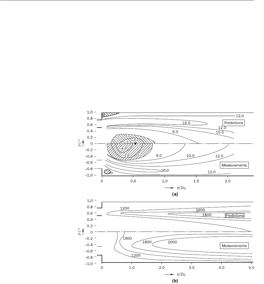
modelling of ﬁres. Figure 3.15 (Jones and Whitelaw, 1982) shows the results

of early calculations with the k–

model of turbulent combusting ﬂows for

an axisymmetric combustor. Computed contours of axial velocity and

temperature are compared with experimental values showing good general

agreement but differences in detail. The ﬂow pattern in the combustor is

dominated by turbulent transport and hence its correct prediction is vitally

important for the development of the ﬂow ﬁeld and the combustion process.

We come back to this issue in Chapter 12 where we examine different

models of turbulent combustion.

Figure 3.15 Comparison

of predictions of k–

model

with measurements in an

axisymmetric combustor:

(a) axial velocity contours;

(b) temperature contours

Source: Jones and Whitelaw (1982)

In spite of the numerous successes, the standard k–

model shows only

moderate agreement in unconﬁned ﬂows. The model is reported not to perform

well in weak shear layers (far wakes and mixing layers), and the spreading

rate of axisymmetric jets in stagnant surroundings is severely overpredicted.

In large parts of these ﬂows the rate of production of turbulent kinetic energy

is much less than the rate of dissipation, and the difﬁculties can only be over-

come by making ad hoc adjustment to model constants C.

Bradshaw et al. (1981) stated that the practice of incorporating the pressure

transport term of the exact k-equation in the gradient diffusion expression of

ANIN_C03.qxd 29/12/2006 04:34PM Page 79

the model equation is deemed to be acceptable on the grounds that the

pressure term is sometimes so small that measured turbulent kinetic energy

budgets balance without it. They noted, however, that many of these meas-

urements contain substantial errors, and it is certainly not generally true that

pressure diffusion effects are negligible.

We can expect that the k–

model, and all other models that are based

on Boussinesq’s isotropic eddy viscosity assumption, will have problems in

swirling ﬂows and ﬂows with large rapid extra strains (e.g. highly curved

boundary layers and diverging passages) that affect the structure of turbu-

lence in a subtle manner. Secondary ﬂows in long non-circular ducts, which

are driven by anisotropic normal Reynolds stresses, can also not be predicted

due to the same deﬁciencies of the treatment of normal stresses within the

k–

model. Finally, the model is oblivious to body forces due to rotation of

the frame of reference.

A summary of the performance assessment for the standard k–

model is

given in Table 3.4.

80 CHAPTER 3 TURBULENCE AND ITS MODELLING

Table 3.4 Standard k–

model assessment

Advantages:

• simplest turbulence model for which only initial and/or boundary

conditions need to be supplied

• excellent performance for many industrially relevant ﬂows

• well established, the most widely validated turbulence model

Disadvantages:

• more expensive to implement than mixing length model (two extra PDEs)

• poor performance in a variety of important cases such as:

(i) some unconﬁned ﬂows

(ii) ﬂows with large extra strains (e.g. curved boundary layers, swirling

ﬂows)

(iii) rotating ﬂows

(iv) ﬂows driven by anisotropy of normal Reynolds stresses (e.g. fully

developed ﬂows in non-circular ducts)

3.7.3 Reynolds stress equation models

The most complex classical turbulence model is the Reynolds stress equa-

tion model (RSM), also called the second-order or second-moment closure

model. Several major drawbacks of the k–

model emerge when it is attempted

to predict ﬂows with complex strain ﬁelds or signiﬁcant body forces. Under

such conditions the individual Reynolds stresses are poorly represented by

formula (3.48) even if the turbulent kinetic energy is computed to reasonable

accuracy. The exact Reynolds stress transport equation on the other hand

can account for the directional effects of the Reynolds stress ﬁeld.

The modelling strategy originates from work reported in Launder et al.

(1975). We follow established practice in the literature and call R

=−

= the Reynolds stress, although the term kinematic Reynolds stress

would be more precise. The exact equation for the transport of R

takes the

following form:

′u

′

ANIN_C03.qxd 29/12/2006 04:35PM Page 80

3.7 RANS EQUATIONS AND TURBULENCE MODELS 81

=+C

= P

+ D

−

+Π

+Ω

(3.55)

Rate of Transport Rate of Transport Rate of Transport of R

due Transport

change of + of R

by = production + of R

by − dissipation + to turbulent pressure + of R

due to

= convection of R

diffusion of R

– strain interactions rotation

Equation (3.55) describes six partial differential equations: one for the trans-

port of each of the six independent Reynolds stresses ( , , , ,

and , since = , = and = ). If it is compared

with the exact transport equation for the turbulent kinetic energy (3.42)

two new physical processes appear in the Reynolds stress equations: the

pressure–strain interaction or correlation term Π

, whose effect on the

kinetic energy can be shown to be zero, and the rotation term Ω

In CFD computations with the Reynolds stress transport equations the

convection, production and rotation terms can be retained in their exact

form. The convective term is as follows:

==div(

U) (3.56)

the production term is

=− R

+ R

(3.57)

and, ﬁnally, the rotational term is given by

Ω

=−2

( e

ikm

+ e

jkm

) (3.58)

Here

is the rotation vector and e

ijk

is the alternating symbol; e

ijk

=+1 if i,

j and k are different and in cyclic order, e

ijk

=−1 if i, j and k are different and

in anti-cyclic order; and e

ijk

= 0 if any two indices are the same.

To obtain a solvable form of (3.55) we need models for the diffusion, the

dissipation rate and the pressure–strain correlation terms on the right hand

side. Launder et al. (1975) and Rodi (1980) gave comprehensive details of

the most general models. For the sake of simplicity we quote those models

derived from this approach that are used in some commercial CFD codes.

These models often lack somewhat in detail, but their structure is easier to

understand and the main message is intact in all cases.

The diffusion term D

can be modelled with the assumption that the rate

of transport of Reynolds stresses by diffusion is proportional to gradients of

Reynolds stresses. This gradient diffusion idea recurs throughout turbulence

modelling. Commercial CFD codes often favour the simplest form:

==div grad(R

) (3.59)

with

= C

, C

= 0.09 and

= 1.0

∂

′u′

∂

′u

′

∂

(

′u

′)

∂

′u

′

′u

′

′u

′

∂

ANIN_C03.qxd 29/12/2006 04:35PM Page 81

82 CHAPTER 3 TURBULENCE AND ITS MODELLING

The dissipation rate

is modelled by assuming isotropy of the small dissi-

pative eddies. It is set so that it affects the normal Reynolds stresses (i = j)

only and each stress component in equal measure. This can be achieved by

εδ

(3.60)

where

is the dissipation rate of turbulent kinetic energy deﬁned by (3.43).

The Kronecker delta

is given by

= 1 if i = j and

= 0 if i ≠ j.

The pressure–strain interactions constitute one of the most important

terms in (3.55), but the most difﬁcult one to model accurately. Their effect

on the Reynolds stresses is caused by two distinct physical processes: (i) a

‘slow’ process that reduces anisotropy of the turbulent eddies due to their

mutual interactions; and (ii) a ‘rapid’ process due to interactions between

turbulent ﬂuctuations and the mean ﬂow strain that produce the eddies such

that the anisotropic production of turbulent eddies is opposed. The overall

effect of both processes is to redistribute energy amongst the normal

Reynolds stresses (i = j) so as to make them more isotropic and to reduce the

Reynolds shear stresses (i ≠ j). The simplest account of the slow process

takes the rate of return to isotropic conditions to be proportional to the

degree of anisotropy a

of the Reynolds stresses (a

= R

−

–

) divided by

a characteristic time scale of the turbulence k/

. The rate of the rapid pro-

cess is taken to be proportional to the production processes that generate the

anisotropy. The simplest representation of the pressure–strain term in the

Reynolds stress transport equation is therefore given by

=−C

− k

) − C

− P

) (3.61)

with C

= 1.8 and C

= 0.6

More advanced accounts include corrections in the second set of brackets in

equation (3.61) to ensure that the model is frame invariant (i.e. the effect is

the same irrespective of the co-ordinate system).

The effect of the pressure–strain term (3.61) is to decrease anisotropy of

Reynolds stresses (i.e. to equalise the normal stresses , and ), but

we have seen in section 3.4 that measurements indicate an increase of the

anisotropy of normal Reynolds stresses in the vicinity of a solid wall due to

damping of ﬂuctuations in the directions normal to the wall. Hence, addi-

tional corrections are needed to account for the inﬂuence of wall proximity

on the pressure–strain terms. These corrections are different in nature from

the wall-damping functions encountered in the k–

model and need to be

applied irrespective of the value of the mean ﬂow Reynolds number. It is

beyond the scope of this introduction to give all this detail. The reader is

directed to a comprehensive model that accounts for all these effects in

Launder et al. (1975).

Turbulent kinetic energy k is needed in the above formulae and can be

found by simple addition of the three normal stresses:

k =

–

+ R

) =

–

( ++)

The six equations for Reynolds stress transport are solved along with a

model equation for the scalar dissipation rate

. Again a more exact form is

′

ANIN_C03.qxd 29/12/2006 04:35PM Page 82

3.7 RANS EQUATIONS AND TURBULENCE MODELS 83

found in Launder et al. (1975), but the equation from the standard k–

model

is used in commercial CFD for the sake of simplicity:

= div grad

+ C

. S

− C

(3.62)

where C

= 1.44 and C

= 1.92

Rate of Transport Transport Rate of Rate of

change + of

by = of

by + production − destruction

convection diffusion of

The usual boundary conditions for elliptic ﬂows are required for the solution

of the Reynolds stress transport equations:

• inlet: speciﬁed distributions of R

and

• outlet and symmetry:

∂

n = 0 and

∂ε

∂

n = 0

• free stream: R

= 0 and

= 0 are given or

∂

n = 0 and

∂ε

∂

n = 0

• solid wall: use wall functions relating R

to either k or u

e.g. = 1.1k, = 0.25k, = 0.66k,

−=0.26k

In the absence of any information, approximate inlet distributions for R

may be calculated from the turbulence intensity T

and a characteristic length

L of the equipment (e.g. equivalent pipe diameter) by means of the follow-

ing assumed relationships:

k = (U

ref

)

= C

3/4

 = 0.07L

= k ==k

= 0 (i ≠ j )

Expressions such as these should not be used without a subsequent test of

the sensitivity of results to the assumed inlet boundary conditions.

For computations at high Reynolds numbers wall-function-type bound-

ary conditions can be used, which are very similar to those of the k–

model

and relate the wall shear stress to mean ﬂow quantities. Near-wall Reynolds

stress values are computed from formulae such as R

==c

k, where the

are obtained from measurements.

Low Reynolds number modiﬁcations to the models can be incorporated

to add the effects of molecular viscosity to the diffusion terms and to account

for anisotropy in the dissipation rate term in the R

-equations. Wall-damping

functions to adjust the constants of the

-equation and Launder and Sharma’s

modiﬁed dissipation rate variable 6 ≡

− 2

(

∂

1/2

∂

(see also section 3.7.2)

give more realistic modelling near solid walls (Launder and Sharma, 1974).

So et al. (1991) gave a review of the performance of near-wall treatments

where details may be found.

Similar models involving three further model PDEs – one for every tur-

bulent scalar ﬂux of equation (3.32) – are available for scalar transport.

′

′u

′

′u

′

3/2



′u

′

ANIN_C03.qxd 29/12/2006 04:35PM Page 83

The interested reader is referred to Rodi (1980) for further material. Com-

mercial CFD codes may use or give as an alternative the simple expedient of

solving a single scalar transport equation and using the Reynolds analogy by

adding a turbulent diffusion coefﬁcient Γ

to the laminar diffusion

coefﬁcient with a speciﬁed value of the Prandtl/Schmidt numbers

around

0.7. Little is known about low Reynolds number modiﬁcations to the scalar

transport equations in near-wall ﬂows.

Assessment of performance

RSMs are clearly quite complex, but it is generally accepted that they are

the ‘simplest’ type of model with the potential to describe all the mean

ﬂow properties and Reynolds stresses without case-by-case adjustment. The

RSM is by no means as well validated as the k–

model, and because of

the high cost of the computations it is not so widely used in industrial ﬂow

calculations (Table 3.5). Moreover, the model can suffer from convergence

problems due to numerical issues associated with the coupling of the mean

velocity and turbulent stress ﬁelds through source terms. The extension and

improvement of these models is an area of very active research. Once a con-

sensus has been reached about the precise form of the component models

and the best numerical solution strategy, it is likely that this form of turbu-

lence modelling will begin to be more widely applied by industrial users.

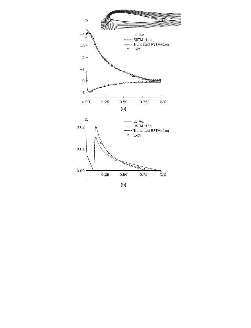
Figure 3.16 (Leschziner, in Peyret and Krause, 2000) gives a performance

comparison of the RSM and k–

models against measured distributions of

pressure coefﬁcient and suction-side skin friction coefﬁcients for an

Aérospatiale aerofoil. Leschziner notes that the aerofoil is close to stall at the

chosen angle of attack. The diagrams show that the k–

model (labelled

LL k–

) fails to reproduce several details of the pressure distribution in the

leading and trailing edge regions. The prediction of the onset of separation

depends crucially on the details of the boundary layer structure just

upstream, which are captured much better by the RSM model (labelled

RSTM + 1eq, to highlight the chosen treatment of the viscous sub-layer).

This model also gives excellent agreement with the measured distribution of

skin friction on the suction side of the aerofoil.

84 CHAPTER 3 TURBULENCE AND ITS MODELLING

Table 3.5 RSM assessment

Advantages:

• potentially the most general of all classical turbulence models

• only initial and/or boundary conditions need to be supplied

• very accurate calculation of mean ﬂow properties and all Reynolds stresses

for many simple and more complex ﬂows including wall jets, asymmetric

channel and non-circular duct ﬂows and curved ﬂows

Disadvantages:

• very large computing costs (seven extra PDEs)

• not as widely validated as the mixing length and k–

models

• performs just as poorly as the k–

model in some ﬂows due to identical

problems with the

-equation modelling (e.g. axisymmetric jets and

unconﬁned recirculating ﬂows)

ANIN_C03.qxd 29/12/2006 04:35PM Page 84

3.7 RANS EQUATIONS AND TURBULENCE MODELS 85

3.7.4 Advanced turbulence models

Two-equation turbulence models, such as the k–

model introduced earlier,

give good results for simple ﬂows and some recirculating ﬂows, but research

over a period of three decades has highlighted a number of shortcomings.

Leschziner (in Peyret and Krause, 2000) and Hanjaliz (2004) summarised

the nature and causes of these performance problems:

• Low Reynolds number ﬂows: in these ﬂows wall functions based on

the log-law are inaccurate and it is necessary to integrate the k- and

-equations to the wall. Very rapid changes occur in the distributions

of k and

as we reach the buffer layer between the fully turbulent

region and the viscous sublayer. This requires large numbers of grid

points to resolve the changes, and we also need non-linear wall-damping

functions to force upon k and

the correct behaviour as the character

of the near-wall ﬂow changes from turbulence dominated to viscous

dominated. As a consequence the system of equations that needs to be

solved is numerically stiff, which means that it may be difﬁcult to get

converged solutions. Furthermore, the results can be grid dependent.

• Rapidly changing ﬂows: the Reynolds stress −

is proportional to the

mean rate of strain S

in two-equation models. This only holds when

′u

′

Figure 3.16 Comparison of

predictions of RSM and standard

k–

model with measurements on

a high-lift Aérospatiale aerofoil:

(a) pressure coefﬁcient; (b) skin

friction coefﬁcient

Source: Leschziner, in Peyret and

Krause (2000)

ANIN_C03.qxd 29/12/2006 04:35PM Page 85

the rates of production and dissipation of turbulence kinetic energy are

roughly in balance. In rapidly changing ﬂows this is not the case.

• Stress anisotropy: the normal Reynolds stresses −

will all be

approximately equal to −

–

k if a thin shear layer ﬂow is evaluated

using a two-equation model. Experimental data presented in section 3.4

showed that this is not correct, but in spite of this the k–

model

performs well in such ﬂows because the gradients of normal turbulent

stresses −

are small compared with the gradient of the dominant

turbulent shear stress −

. Consequently, the normal stresses may be

large, but they are not dynamically active in thin shear layer ﬂows, i.e.

they are not responsible for driving any ﬂows. In more complex ﬂows

the gradients of normal turbulent stresses are not negligible and can

drive signiﬁcant ﬂows. These effects cannot be predicted by the

standard two-equation models.

• Strong adverse pressure gradients and recirculation regions: this problem

particularly affects the k–

model and is also attributable to the isotropy

of its predicted normal Reynolds stresses and the resultant failure to

represent correctly the subtle interactions between normal Reynolds

stresses and mean ﬂow that determine turbulent energy production.

The k–

model overpredicts the shear stress and suppresses separation

in ﬂows over curved walls. This is a signiﬁcant problem in ﬂows over

aerofoils, e.g. in aerospace applications.

• Extra strains: streamline curvature, rotation and extra body forces all

give rise to additional interactions between the mean strain rate and the

Reynolds stresses. These physical effects are not captured by standard

two-equation models.

As we have seen, the RSM incorporates an exact representation of the

Reynolds stress production process and, hence, addresses most of these

problems adequately, but at the cost of a signiﬁcant increase in computer

storage and run time. Below we consider some of the more recent advances

in turbulence modelling that seek to address some or all of the above

problems.

Advanced treatment of the near-wall region: two-layer k---

εε

model

The two-layer model represents an improved treatment of the near-wall

region for turbulent ﬂows at low Reynolds number. The intention is, as

in the low Reynolds number k–

model discussed earlier, to integrate to

the wall by placing the near-wall grid point in the viscous sublayer ( y

< 1).

The numerical stability problems (Chen and Patel, 1988) associated with the

non-linear wall-damping functions, necessary in the low Reynolds number

k–

model to integrate both k- and

-equations to the wall, are avoided by

sub-dividing the boundary layer into two regions (Rodi, 1991):

• Fully turbulent region, Re

= yk/

≥ 200: the standard k–

model is

used and the eddy viscosity is computed with the usual relationship

(3.44),

t,t

= C

• Viscous region, Re

< 200: only the k-equation is solved in this

region and a length scale is speciﬁed using  =

y[1 − exp(−Re

/A)]

for the evaluation of the rate of dissipation with

= C

3/4

3/2

/ using

A = 2

−3/4

and the eddy viscosity in this region with

t,v

= C

1/4

k 

and A = 70

u′v′

′

86 CHAPTER 3 TURBULENCE AND ITS MODELLING

ANIN_C03.qxd 29/12/2006 04:35PM Page 86