Versteeg H., Malalasekra W. An Introduction to Computational Fluid Dynamics: The Finite Volume Method

Подождите немного. Документ загружается.

3.7 RANS EQUATIONS AND TURBULENCE MODELS 67

No. of extra transport equations Name

Zero Mixing length model

One Spalart–Allmaras model

Two k–

model

k–

model

Algebraic stress model

Seven Reynolds stress model

These models form the basis of standard turbulence calculation procedures

in currently available commercial CFD codes.

Eddy viscosity and eddy diffusivity

Of the tabulated models the mixing length and k–

models are at present by

far the most widely used and validated. They are based on the presumption

that there exists an analogy between the action of viscous stresses and

Reynolds stresses on the mean ﬂow. Both stresses appear on the right hand

side of the momentum equation, and in Newton’s law of viscosity the viscous

stresses are taken to be proportional to the rate of deformation of ﬂuid

elements. For an incompressible ﬂuid this gives

+ (2.31)

In order to simplify the notation the so-called sufﬁx notation has been used

here. The convention of this notation is that i or j = 1 corresponds to the

x-direction, i or j = 2 the y-direction and i or j = 3 the z-direction. So, for

example,

In section 3.4 we reviewed experimental evidence which showed that turbu-

lence decays unless there is shear in isothermal incompressible ﬂows. Further-

more, turbulent stresses are found to increase as the mean rate of deformation

increases. Boussinesq proposed in 1877 that Reynolds stresses might be

proportional to mean rates of deformation. Using the sufﬁx notation we get

=−

+−

(3.33)

where k =

–

( ++) is the turbulent kinetic energy per unit mass (see

section 3.3).

The ﬁrst term of the right hand side is analogous to formula (2.31) above

except for the appearance of the turbulent or eddy viscosity

(dimensions

Pa s). There is also a kinematic turbulent or eddy viscosity denoted by

with dimensions m

/s. The second term on the right hand side involves

the Kronecker delta (

= 1 if i = j and

= 0 if i ≠ j). This contribution

ensures that the formula gives the correct result for the normal Reynolds

w′

v′

u′

∂

′u

′

∂

ANIN_C03.qxd 29/12/2006 04:34PM Page 67

stresses (those with i = j), and hence for

=−

and

=−

. To demonstrate the necessity of the extra term we consider an

incompressible ﬂow and explore the behaviour of the ﬁrst part of (3.33) by

itself. If we sum this over all the normal stresses (i.e. let i = 1, 2 and 3 whilst

keeping i = j ) we ﬁnd, using continuity, that it is zero, since

= 2

++ =2

div U = 0

Clearly in any ﬂow the sum of the normal stresses −

( ++) is equal

to minus twice the turbulence kinetic energy per unit volume (−2

k). In

equation (3.33) an equal third is allocated to each normal stress component

to ensure their sum always has its physically correct value. It should be noted

that this implies an isotropic assumption for the normal Reynolds stresses

which the data in section 3.4 have shown is inaccurate even in simple two-

dimensional ﬂows.

Turbulent transport of heat, mass and other scalar properties can be mod-

elled similarly. Formula (3.33) shows that turbulent momentum transport is

assumed to be proportional to mean gradients of velocity (i.e. gradients of

momentum per unit mass). By analogy turbulent transport of a scalar is taken

to be proportional to the gradient of the mean value of the transported quan-

tity. In sufﬁx notation we get

−

=Γ

(3.34)

where Γ

is the turbulent or eddy diffusivity.

Since turbulent transport of momentum and heat or mass is due to the

same mechanism – eddy mixing – we expect that the value of the turbulent

diffusivity Γ

is fairly close to that of the turbulent viscosity

. This assump-

tion is better known as the Reynolds analogy. We introduce a turbulent

Prandtl/Schmidt number deﬁned as follows:

= (3.35)

Experiments in many ﬂows have established that this ratio is often nearly

constant. Most CFD procedures assume this to be the case and use values of

around unity.

Preamble

It has become clear from our discussions of simple turbulent ﬂows in section

3.4 that turbulence levels and turbulent stresses vary from point to point in

a ﬂow. Mixing length models attempt to describe the stresses by means of

simple algebraic formulae for

as a function of position. The k–

εε

model is

a more sophisticated and general, but also more costly, description of turbu-

lence which allows for the effects of transport of turbulence properties by

convection and diffusion and for production and destruction of turbulence.

Two transport equations (PDEs), one for the turbulent kinetic energy k and

a further one for the rate of dissipation of turbulent kinetic energy

, are solved.

The underlying assumption of both these models is that the turbulent

viscosity

is isotropic: in other words that the ratio between Reynolds stress

∂

′

w′

v′

u′

∂

w′

v′

u′

68 CHAPTER 3 TURBULENCE AND ITS MODELLING

ANIN_C03.qxd 29/12/2006 04:34PM Page 68

3.7 RANS EQUATIONS AND TURBULENCE MODELS 69

and mean rate of deformation is the same in all directions. This assumption

fails in many complex ﬂows where it leads to inaccurate predictions. Here it

is necessary to derive and solve transport equations for the Reynolds stresses

themselves. It may at ﬁrst seem strange to think that a stress can be subject

to transport. However, it is only necessary to remember that the Reynolds

stresses initially appeared on the left hand side of the momentum equations

and are physically due to convective momentum exchanges as a consequence

of turbulent velocity ﬂuctuations. Fluid momentum – mean momentum as

well as ﬂuctuating momentum – can be transported by ﬂuid particles and

therefore the Reynolds stresses can also be transported.

The six transport equations, one for each Reynolds stress, contain diffu-

sion, pressure–strain and dissipation terms whose individual effects are

unknown and cannot be measured. In Reynolds stress equation models

(also known in the literature as second-order or second-moment closure

models) assumptions are made about these unknown terms, and the result-

ing PDEs are solved in conjunction with the transport equation for the rate

of dissipation of turbulent kinetic energy

. The design of Reynolds stress

equation models is an area of vigorous research, and the models have not

been validated as widely as the mixing length and k–

model. Solving the

seven extra PDEs gives rise to a substantial increase in the cost of CFD sim-

ulations when compared with the k–

model, so the application of Reynolds

stress equation models outside the academic fraternity is relatively recent.

A much more far-reaching set of modelling assumptions reduces the

PDEs describing Reynolds stress transport to algebraic equations to be

solved alongside the k and

equations of the k–

model. This approach leads

to the algebraic stress models that are the most economical form of

Reynolds stress model able to introduce anisotropic turbulence effects into

CFD simulations.

In the following sections the mixing length and k–

models will be dis-

cussed in detail and the main features of the Reynolds stress equation and

algebraic stress models will be outlined. We also describe the k–

ωω

models

and the Spalart–Allmaras model, which are more recent entrants to the

industrial CFD arena, and outline the distinguishing features of other models

that are beginning to make an impact on industrial turbulence modelling.

3.7.1 Mixing length model

On dimensional grounds we assume the kinematic turbulent viscosity

which has dimensions m

/s, can be expressed as a product of a turbulent

velocity scale

(m/s) and a turbulent length scale  (m). If one velocity scale

and one length scale sufﬁce to describe the effects of turbulence, dimensional

analysis yields

= C

 (3.36)

where C is a dimensionless constant of proportionality. Of course the

dynamic turbulent viscosity is given by

= C

ρϑ



Most of the kinetic energy of turbulence is contained in the largest eddies,

and turbulence length scale  is therefore characteristic of these eddies which

interact with the mean ﬂow. If we accept that there is a strong connection

ANIN_C03.qxd 29/12/2006 04:34PM Page 69

70 CHAPTER 3 TURBULENCE AND ITS MODELLING

Table 3.2 Mixing lengths for two-dimensional turbulent ﬂows

Flow Mixing length 

Mixing layer 0.07L Layer width

Jet 0.09L Jet half width

Wake 0.16L Wake half width

Axisymmetric jet 0.075L Jet half width

Boundary layer (

∂

x = 0)

viscous sub-layer and

y[1 − exp(−y

/26)]

log-law layer ( y/L ≤ 0.22) Boundary layer

outer layer ( y/L ≥ 0.22) 0.09L thickness

Pipes and channels Pipe radius or

(fully developed ﬂow) L

[0.14–0.08(1 − y/L)

− 0.06(1 − y/L)

] channel half width

between the mean ﬂow and the behaviour of the largest eddies we can

attempt to link the characteristic velocity scale of the eddies with the mean

ﬂow properties. This has been found to work well in simple two-dimensional

turbulent ﬂows where the only signiﬁcant Reynolds stress is

=−

and the only signiﬁcant mean velocity gradient is

∂

y. For such ﬂows it is

at least dimensionally correct to state that, if the eddy length scale is ,

= c  (3.37)

where c is a dimensionless constant. The absolute value is taken to ensure

that the velocity scale is always a positive quantity irrespective of the sign of

the velocity gradient.

Combining (3.36) and (3.37) and absorbing the two constants C and c into

a new length scale 

we obtain

= 

(3.38)

This is Prandtl’s mixing length model. Using formula (3.33) and noting

that

∂

y is the only signiﬁcant mean velocity gradient, the turbulent

Reynolds stress is described by

=−



(3.39)

Turbulence is a function of the ﬂow, and if the turbulence changes it is

necessary to account for this within the mixing length model by varying 

For a substantial category of simple turbulent ﬂows, which includes the

free turbulent ﬂows and wall boundary layers discussed in section 3.4,

the turbulence structure is sufﬁciently simple that 

can be described by

means of simple algebraic formulae. Some examples are given in Table 3.2

(Rodi, 1980).

∂

u′v′

∂

u′v′

ANIN_C03.qxd 29/12/2006 04:34PM Page 70

3.7 RANS EQUATIONS AND TURBULENCE MODELS 71

The mixing length model can also be used to predict turbulent transport

of scalar quantities. The only turbulent transport term which matters in the

two-dimensional ﬂows for which the mixing length is useful is modelled as

follows:

−

=Γ

(3.40)

where Γ

and

ρν

where

is found from (3.38). Rodi (1980)

recommended values for

of 0.9 in near-wall ﬂows, 0.5 for jets and mixing

layers and 0.7 in axisymmetric jets.

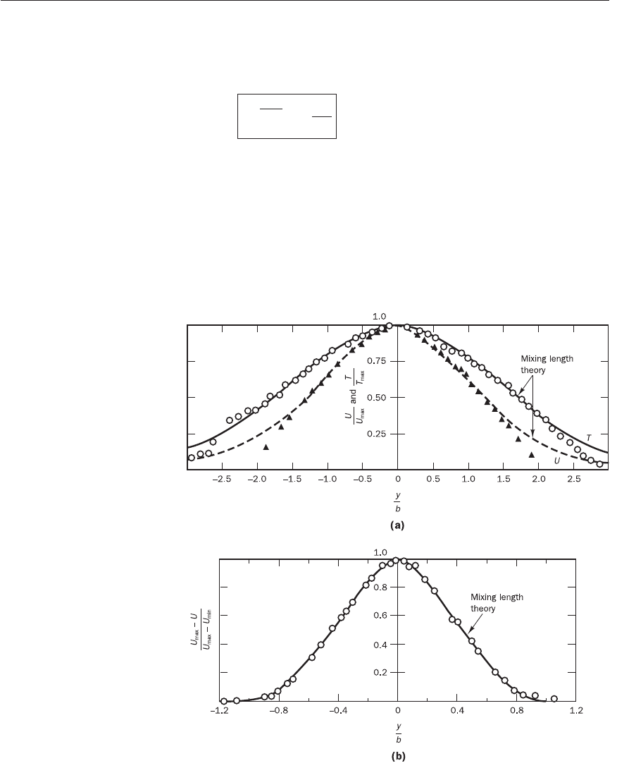
In the formulae in Table 3.2 y represents the distance from the wall and

= 0.41 is von Karman’s constant. The expressions give very good agree-

ment between computed results and experiments for mean velocity distribu-

tions, wall friction coefﬁcients and other ﬂow properties such as heat transfer

coefﬁcients in simple two-dimensional ﬂows. Results for two ﬂows from

Schlichting (1979) are given below in Figures 3.14a–b.

∂

v′

′

Figure 3.14 Results of

calculations using mixing

length model for (a) planar jet

and (b) wake behind a long,

slender, circular cylinder

Source: Schlichting, H. (1979)

Boundary Layer Theory, 7th edn,

reproduced with permission of

The McGraw-Hill Companies

The mixing length has been found to be very useful in simple two-

dimensional ﬂows with slow changes in the ﬂow direction. In these cases

the production of turbulence is in balance with its dissipation throughout

ANIN_C03.qxd 29/12/2006 04:34PM Page 71

the ﬂow, and turbulence properties develop in proportion with a mean ﬂow

length scale L. This means that in such ﬂows the mixing length 

is pro-

portional to L and can be described as a function of position by means of

a simple algebraic formula. The majority of practically important ﬂows,

however, involve additional contributions to the budgets of turbulence

properties due to transport, i.e. convection and diffusion. Moreover, the

production and destruction processes may be modiﬁed by the ﬂow itself.

Consequently, the mixing length model is not used on its own in general-

purpose CFD, but we will ﬁnd it embedded in many of the more sophisti-

cated turbulence models to describe near-wall ﬂow behaviour as part of the

treatment of wall boundary conditions.

An overall assessment of the mixing length model is given in Table 3.3.

72 CHAPTER 3 TURBULENCE AND ITS MODELLING

Table 3.3 Mixing length model assessment

Advantages:

• easy to implement and cheap in terms of computing resources

• good predictions for thin shear layers: jets, mixing layers, wakes and

boundary layers

• well established

Disadvantages:

• completely incapable of describing ﬂows with separation and recirculation

• only calculates mean ﬂow properties and turbulent shear stress

3.7.2 The k---

εε

model

In two-dimensional thin shear layers the changes in the ﬂow direction are

always so slow that the turbulence can adjust itself to local conditions. In ﬂows

where convection and diffusion cause signiﬁcant differences between produc-

tion and destruction of turbulence, e.g. in recirculating ﬂows, a compact

algebraic prescription for the mixing length is no longer feasible. The way

forward is to consider statements regarding the dynamics of turbulence. The

k–

model focuses on the mechanisms that affect the turbulent kinetic energy.

Some preliminary deﬁnitions are required ﬁrst. The instantaneous kinetic

energy k(t) of a turbulent ﬂow is the sum of the mean kinetic energy K =

–

+ V

+ W

) and the turbulent kinetic energy k =

–

( ++):

k(t) = K + k

In the developments below we extensively need to use the rate of deforma-

tion and the turbulent stresses. To facilitate the subsequent calculations it is

common to write the components of the rate of deformation s

and the

stresses

in tensor (matrix) form:

= Hs

K and

= H

Decomposition of the rate of deformation of a ﬂuid element in a turbulent

ﬂow into a mean and a ﬂuctuating component, s

(t) = S

+ s′

, gives the fol-

lowing matrix elements:

w′

v′

u′

ANIN_C03.qxd 29/12/2006 04:34PM Page 72

3.7 RANS EQUATIONS AND TURBULENCE MODELS 73

(t) = S

+ s′

=+ s

(t) = S

+ s′

(t) = S

+ s′

(t) = S

+ s′

= s

(t) = S

+ s′

=+++

(t) = S

+ s′

= s

(t) = S

+ s′

=+++

(t) = S

+ s′

= s

(t) = S

+ s′

=+++

The product of a vector a and a tensor b

is a vector c whose components can

be calculated by application of the ordinary rules of matrix algebra:

JGa

+ a

≡ a

= [a

] Hb

K = Ha

+ a

K = Hc

= c

LIa

+ a

LIc

The scalar product of two tensors a

and b

is evaluated as follows:

. b

= a

+ a

We have used the convention of the sufﬁx notation where the x-direction

is denoted by subscript 1, the y-direction by 2 and the z-direction by 3.

It can be seen that products are formed by taking the sum over all possible

values of every repeated sufﬁx.

Governing equation for mean flow kinetic energy K

An equation for the mean kinetic energy K can be obtained by multiplying

x-component Reynolds equation (3.27a) by U, y-component equation

(3.27b) by V and z-component equation (3.27c) by W. After adding together

the results and a fair amount of algebra it can be shown that the time-

average equation governing the mean kinetic energy of the ﬂow is as follows

(Tennekes and Lumley, 1972):

+ div(

KU) = div(−PU + 2

−

U ) − 2

. S

(3.41)

(I) (II) (III) (IV) (V) (VI) (VII)

Or in words

Rate of change Transport Transport

Transport Transport Rate of Rate of destruction

of mean kinetic + of K by = of K by +

of K by

−

viscous

−

of K due to

energy K convection pressure

viscous Reynolds dissipation turbulence

stresses stress of K production

The transport terms (III), (IV) and (V) are all characterised by the appearance

of div and it is common practice to place them together inside one pair of

′u

′

∂

(

∂

w′

∂

v′

∂

w′

∂

u′

∂

v′

∂

u′

∂

w′

∂

v′

∂

u′

∂

ANIN_C03.qxd 29/12/2006 04:34PM Page 73

74 CHAPTER 3 TURBULENCE AND ITS MODELLING

brackets. The effects of the viscous stresses on K have been split into two parts:

term (IV), the transport of K due to viscous stresses; and term (VI), the viscous

dissipation of mean kinetic energy K. The two terms that contain the Reynolds

stresses −

account for turbulence effects: term (V) is the turbulent

transport of K by means of Reynolds stresses and (VII) is the net decrease of

K due to deformation work by Reynolds stresses giving rise to turbulence

production. In high Reynolds number ﬂows the turbulent terms (V) and

(VII) are always much larger than their viscous counterparts (IV) and (VI).

Governing equation for turbulent kinetic energy k

Multiplication of each of the instantaneous Navier–Stokes equations (3.24a–c)

by the appropriate ﬂuctuating velocity components (i.e. x-component equa-

tion multiplied by u′ etc.) and addition of all the results, followed by a repeat

of this process on the Reynolds equations (3.27a–c), subtraction of the two

resulting equations and very substantial rearrangement, yields the equation

for turbulent kinetic energy k (Tennekes and Lumley, 1972).

+ div(

kU) = div(−+2

−

–

) − 2

−

. S

(3.42)

(I) (II) (III) (IV) (V) (VI) (VII)

In words

Rate of change of Transport Transport Transport of Transport of Rate of Rate of

turbulent kinetic + of k by = of k by + k by viscous + k by Reynolds − dissipation + production

energy k convection pressure stresses stress of k of k

Equations (3.41) and (3.42) look very similar in many respects; however, the

appearance of primed quantities on the right hand side of the k-equation

shows that changes to the turbulent kinetic energy are mainly governed by

turbulent interactions. Terms (VII) in both equations are equal in magni-

tude, but opposite in sign. In two-dimensional thin shear layers we found

(see section 3.4) that the only signiﬁcant Reynolds stress −

is usually

positive if the main term of S

in such a ﬂow, the mean velocity gradient

∂

y, is positive. Hence term (VII) gives a positive contribution in the

k-equation and represents a production term. In the K-equation, however,

the sign is negative, so there the term destroys mean ﬂow kinetic energy.

This expresses mathematically the conversion of mean kinetic energy into

turbulent kinetic energy.

The viscous dissipation term (VI),

−2

=−2

( +++2 + 2 + 2)

gives a negative contribution to (3.42) due to the appearance of the sum

of squared ﬂuctuating deformation rates s′

. The dissipation of turbulent

kinetic energy is caused by work done by the smallest eddies against viscous

stresses. The rate of dissipation per unit volume (VI) is normally written as

the product of the density

and the rate of dissipation of turbulent kinetic

energy per unit mass

, so

= 2

(3.43)

s′

. s ′

s′

. s ′

u′v′

′u

′s′

. s′

′ . u

′u

′u′s′

p′u′

∂

(

∂

′u

′

ANIN_C03.qxd 29/12/2006 04:34PM Page 74

3.7 RANS EQUATIONS AND TURBULENCE MODELS 75

The dimensions of

are m

. This quantity is of vital importance in the

study of turbulence dynamics. It is the destruction term in the turbulent

kinetic energy equation, of a similar order of magnitude as the production

term and never negligible. When the Reynolds number is high, the viscous

transport term (IV) in (3.42) is always very small compared with the turbu-

lent transport term (V) and the dissipation (VI).

The k---

εε

model equations

It is possible to develop similar transport equations for all other turbulence

quantities including the rate of viscous dissipation

(see Bradshaw et al.,

1981). The exact

-equation, however, contains many unknown and unmea-

surable terms. The standard k–

εε

model (Launder and Spalding, 1974) has

two model equations, one for k and one for

, based on our best understand-

ing of the relevant processes causing changes to these variables.

We use k and

to deﬁne velocity scale

and length scale  representative

of the large-scale turbulence as follows:

= k

1/2

 =

One might question the validity of using the ‘small eddy’ variable

to deﬁne

the ‘large eddy’ scale . We are permitted to do this because at high Reynolds

numbers the rate at which large eddies extract energy from the mean ﬂow is

broadly matched to the rate of transfer of energy across the energy spectrum

to small, dissipating, eddies if the ﬂow does not change too rapidly. If this

was not the case the energy at some scales of turbulence could grow or

diminish without limit. This does not occur in practice and justiﬁes the use

in the deﬁnition of .

Applying dimensional analysis we can specify the eddy viscosity as

follows:

= C

ρϑ

 =

(3.44)

where C

is a dimensionless constant.

The standard k–

model uses the following transport equations for k

and

+ div(

kU) = div grad k + 2

. S

−

ρε

(3.45)

+ div(

ρε

U) = div grad

+ C

. S

− C

(3.46)

In words the equations are

Rate of Transport Transport Rate of Rate of

change of + of k or

by = of k or

+ production − destruction

k or

convection by diffusion of k or

of k or

∂

(

ρε

)

∂

(

∂

3/2

ANIN_C03.qxd 29/12/2006 04:34PM Page 75

76 CHAPTER 3 TURBULENCE AND ITS MODELLING

The equations contain ﬁve adjustable constants: C

, C

and C

. The

standard k–

model employs values for the constants that are arrived at by

comprehensive data ﬁtting for a wide range of turbulent ﬂows:

= 0.09

= 1.00

= 1.30 C

= 1.44 C

= 1.92 (3.47)

The production term in the model k-equation is derived from the exact

production term in (3.42) by substitution of (3.33). A modelled form of the

principal transport processes in the k- and

-equation appears on the right

hand side. The turbulent transport terms are represented using the gradient

diffusion idea introduced earlier in the context of scalar transport (see equa-

tion (3.34)). Prandtl numbers

and

connect the diffusivities of k and

to the eddy viscosity

. The pressure term (III) of the exact k-equation can-

not be measured directly. Its effect is accounted for in equation (3.45) within

the gradient diffusion term.

Production and destruction of turbulent kinetic energy are always closely

linked. Dissipation rate

is large where production of k is large. The model

equation (3.46) for

assumes that its production and destruction terms are

proportional to the production and destruction terms of the k-equation

(3.45). Adoption of such forms ensures that

increases rapidly if k increases

rapidly and that it decreases sufﬁciently fast to avoid (non-physical) negative

values of turbulent kinetic energy if k decreases. The factor

/k in the pro-

duction and destruction terms makes these terms dimensionally correct in

the

-equation. Constants C

and C

allow for the correct proportionality

between the terms in the k- and

-equations.

To compute the Reynolds stresses we use the familiar Boussinesq

relationship:

−

+−

= 2

−

(3.48)

Boundary conditions

The model equations for k and

are elliptic by virtue of the gradient diffu-

sion term. Their behaviour is similar to the other elliptic ﬂow equations,

which gives rise to the need for the following boundary conditions:

• inlet: distributions of k and

must be given

• outlet, symmetry

axis:

∂

n = 0 and

∂ε

∂

n = 0

• free stream: k and

must be given or

∂

n = 0 and

∂ε

∂

n = 0

• solid walls: approach depends on Reynolds number (see below)

In exploratory design calculations the detailed boundary condition informa-

tion required to operate the model may not be available. Industrial CFD

users rarely have measurements of k and

at their disposal. Progress can

be made by entering values of k and

from the literature (e.g. publications

referred to in section 3.4) and subsequently exploring the sensitivity of the

results to these inlet distributions. If no information is available at all, rough

approximations for the inlet distributions for k and

in internal ﬂows can

be obtained from the turbulence intensity T

and a characteristic length L of

∂

′u

′

ANIN_C03.qxd 29/12/2006 04:34PM Page 76