Zhang K., Li D. Electromagnetic Theory for Microwaves and Optoelectronics
Подождите немного. Документ загружается.


10.6 Eigenwave Expansions of Electromagnetic Fields 661
where
F (k
ρ
) =
Z
∞
0
ψ
0
(ρ
0
)J
0
(k
ρ
ρ
0
)ρ
0
dρ
0
= H
−1
0
[ψ
0
(ρ
0
)], (10.177)
where H
−1
0
represents inverse Hankel transformation of the zeroth order.
Substitution of (10.177) into (10.175) yields
ψ(ρ, z) =
Z
∞
0
H
−1
0
[ψ
0
(ρ
0
)]J
0
(k
ρ
ρ) exp
³
−j
p
k
2
− k
2
z
z
´
k
ρ
dk
ρ
= H
0
n
H
−1
0
[ψ
0
(ρ
0
)] exp
³
−j
q
k
2
− k
2
ρ
z
´o
, (10.178)
where H
0
represents the Hankel transformation of the zeroth order. Within
the paraxial condition (10.178) can be expressed as
ψ(ρ, z) = e
−jkz
H
0
(
H
−1
0
[ψ
0
(ρ
0
)] exp
Ã
jk
2
ρ
z
2k
!)
. (10.179)
As an example, we apply it to obtain the distribution of a Gaussian beam.
Since the Gaussian beam is the solution of a wave equation within the paraxial
condition, here we use this condition too. At z = 0, the field distribution is
assumed to be a function of Gaussian form:
ψ(ρ
0
) = A exp
µ
−ρ
02
w
2
0
, (10.180)
where A is a constant. With normalization the value of A is
A =
r
2
π
1
w
0
. (10.181)
Substitution of (10.180) into (10.177) yields
F (k
ρ
) =
r
2
π
1
w
0
Z
∞
0
exp
µ
−ρ
02
w
2
0
J
0
(k
ρ
ρ
0
)ρ
0
dρ
0
. (10.182)
By the serial expression of the Bessel function,
J
0
(k
ρ
ρ
0
) =
∞
X
n=0
(−1)
n
(n!)
2
µ
k
ρ
ρ
0
2
2n
, (10.183)
(10.182) is expressed as
F (k
ρ
) =
r
2
π
1
w
0
∞
X
n=0
(−1)
n
(n!)
2
µ
k
ρ
2
2n
Z
∞
0
ρ
02n
exp
µ
−ρ
02
w
2
0
ρ
0
dρ
0
=
r
2
π
∞
X
n=0
(−1)
n
w
0
2n!
µ
k
ρ
w
0
2
2n
. (10.184)

662 10. Scalar Diffraction Theory
In deriving (10.184), the integral
Z
∞
0
e
−t
t
n
dt = n! (10.185)
has been used. Introducing the formula that
e
−t
=
∞
X
n=0
(−1)
n
t
n
n!
, (10.186)
We find (10.184) becomes
F (k
ρ
) =
r
1
2π
w
0
exp
"
−
µ
k
ρ
w
0
2
2
#
. (10.187)
Substitution of (10.187) into (10.175) yields the field distribution
ψ (ρ, z) = e
−jkz
Z
∞
0
F (k
ρ
)J
0
(k
ρ
ρ) exp
Ã
jk
2
ρ
z
2k
!
k
ρ
dk
ρ
=
r
1
2π
e
−jkz
w
0
∞
X
n=0
(−1)
n
(n!)
2
Z
∞
0
µ
k
ρ
ρ
2
2n
exp
"
−
µ
k
ρ
w
0
2
2
+
jk
2
ρ
z
2k
#
k
ρ
dk
ρ
.
(10.188)
Introducing (10.185) and (10.186) into (10.188), we obtain after some ma-
nipulation
ψ(ρ, z) =
r
2
π
1
w
exp
µ
−
ρ
2
w
2
exp
·
−jk
µ
z +
ρ
2
2R
+ jφ
¸
. (10.189)
where
w = w
0
r
1 +
³
z
s
´
2
, s =
kw
2
0
2
,
R =
z
2
+ s
2
z
, φ = arctan
³
z
s
´
.
Expression (10.189) represents the distribution of a Gaussian beam, which is
exactly the same as that directly obtained from the paraxial wave equation
in the last chapter.
10.6.3 Eigenmode Expansion in Inhomogeneous Media
In studying the propagation and diffraction of the electromagnetic waves,
the approaches of variable separation and the Green function can only solve
the problems in homogenous media or in media with very simple transverse

10.6 Eigenwave Expansions of Electromagnetic Fields 663
refractive index distribution, such as the field distribution in media with a
quadratic index profile. Even the methods of finite element can only be ap-
plied to the propagation problems in media that are homogeneous in the
longitudinal direction and inhomogeneous in transverse directions. Whereas
with the eigenmode expansion we can treat the propagation of electromag-
netic waves in media with an arbitrary index distribution. In this subsection
we will discuss this approach and the conditions of its application. In fact, in
most cases the variation of the indices is slow, and we will use this condition
in the following discussion.
In inhomogeneous media, the Maxwell equations are
∇ × E = −µ
0
∂H
∂t
, ∇ · [²(x)E] = 0,
∇ × H = ²(x)
∂E
∂t
, ∇ · H = 0,
where ²(x) is a function of spatial coordinates. For the monochromatic wave
we derive
∇
2
E + k
2
E + ∇
µ
E ·
∇²
²
= 0, (10.190)
where k
2
= ω
2
²µ
0
. As ²(x) is a slowly varying function, the third term in
(10.190) is approximately expressed as
∇
µ
E ·
∇²
²
≈ −jE
µ
k ·
∇²
²
. (10.191)
As |∇²/²| ¿ k, this term can b e neglected. This condition is always satisfied
in media such as optical fibers and optical waveguides, so (10.190) is simplified
to
∇
2
E + k
2
E = 0. (10.192)
As the dimensions of the distributing region are much larger than the wave-
length, (10.192) can be solved with scalar theory, and we have
∇
2
E + k
2
E = 0, (10.193)
where E represents a field component. The solution of (10.193) is assumed
to be
E = E
0
exp
·
−j
µ
k
x
x + k
y
y +
Z
z
z
0
k
z
dz
¶¸
, (10.194)
where k
x
and k
y
can be taken as arbitrary real numbers, and k
z
= (k
2
−
k
2
x
− k
2
y
)
1/2
, which is a function of spatial coordinates. Generally k can be
a complex number, which means that the medium may have loss or gain. If
the field distribution at the plane z = z
0
is known, the distribution at plane

664 10. Scalar Diffraction Theory
z = z
0
+ ∆z can be obtained through (10.169),
ψ(x, y, z) =
1
2π
Z
∞
−∞
Z
∞
−∞
F
−1
[ψ
0
(x
0
, y
0
z
0
)]
exp
·
−j
µ
k
x
x + k
y
y +
Z
z
z
0
k
z
dz
¶¸
dk
x
dk
y
, (10.195)
where ψ
0
(x
0
, y
0
z
0
) is the field distribution at the plane z = z
0
. Substituting
the paraxial condition that k
z
= k − (k
2
x
+ k
2
y
)/(2k) into (10.195), we obtain
ψ(x, y, z) =
1
2π
exp
µ
−j
Z
z
z
0
kdz
Z
∞
−∞
Z
∞
−∞
F
−1
[ψ
0
(x
0
, y
0
z
0
)]
exp
Ã
j
Z
z
z
0
k
2
x
+ k
2
y
2k
dz
!
exp[−j(k
x
x + k
y
y)]dk
x
dk
y
. (10.196)
Since ∆z is very small, (10.196) can be expressed as
ψ(x, y, z) =
1
2π
exp
µ
−j
Z
z
z
0
kdz
Z
∞
−∞
Z
∞
−∞
F
−1
[ψ
0
(x
0
, y
0
z
0
)]
exp
"
j(z − z
0
)
¡
k
2
x
+ k
2
y
¢
2k
#
exp[−j(k
x
x + k
y
y)]dk
x
dk
y
. (10.197)
The integral in (10.197) is not a Fourier transformation, since the factor
k in the exponential term is a function of x and y. In most applications, the
spatial variation of the dielectric constant is small and can be expressed as
² = ²
s
+ δ², and accordingly k = k
s
+ δk. (10.198)
Replacing k with k
s
in (10.197), we can express it as a Fourier transformation,
ψ(x, y, z) = exp[−jk(z − z
0
)]F
(
F
−1
[ψ
0
(x
0
, y
0
z
0
)] exp
"
j(z−z
0
)
¡
k
2
x
+ k
2
y
¢
2k
s
#)
.
(10.199)
In the following, we discuss the condition under which k may be replaced
with k
s
. Equation (10.199) can be rewritten as
1
k
=
1
k
s
−
δk
k
2
s
. (10.200)
Then the exponential factor in the middle term of (10.197) is expressed as
j∆z(k
2
x
+ k
2
y
)
2k
=
j∆z
¡
k
2
x
+ k
2
y
¢
2k
s
−
j∆zδk
¡
k
2
x
+ k
2
y
¢
2k
2
s
. (10.201)
The second term on the right-hand side is much smaller than the first term,
but this does not mean that it can be neglected. Only when the phase shift
10.6 Eigenwave Expansions of Electromagnetic Fields 665
Figure 10.23: Coordinate system for the eigenmode expansion of plane wave
in uniaxial crystal.
caused by it is much less than 2π can it be omitted. In other word, only when
∆z is very small can k be replaced with k
s
. For example, in a single-mode
fiber, |δk/k
s
| < 0.005 and (k
2
x
+ k
2
y
)/k
s
< 0.01k
s
. Substituting these into
the second term on the right of (10.201), we obtain ∆zδk(k
2
x
+ k
2
y
)/(2k
2
s
) <
5 × 10
−5
π∆z/λ. If ∆z < 100λ, the value of this term is less than 0.016 and
can be omitted. In fact, to assure high accuracy, we often make ∆z much
less than this value.
From the distribution at the plane z = z
0
, we can derive the distribution at
the plane z = z
0
+∆z. Continuing this process, we can obtain the distribution
in the whole space. This approach is also applied to calculations of the
distribution of the eigenmode in a single-mode waveguide. First, arbitrarily
assign the field distribution at a cross plane. Then repeat the above process
until the field distribution does not change. The final unchanged distribution
is that of the guiding eigenmode in the waveguide.
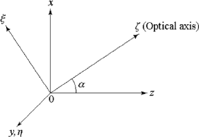
10.6.4 Eigenmode Expansion in Anisotropic Media
In this subsection we discuss the eigenmode expansion of an extraordinary
plane wave in a uniaxial crystal. In Figure 10.23, the field distribution is
known at the plane where z = 0, and from it we are able to derive the field
everywhere. We take ξηζ as the principal coordinate system, and the optical
axis is along the ζ axis. The angle between the ζ axis and the z axis is α.
For an arbitrary field distribution at the plane where z = 0, we do not
know and do not need to know the propagation direction of the wave in
advance. The formulas involved are still (10.164)–(10.169), but the relation
between k
z
and k
x
, k
y
needs to be determined. The transforming relations
for the wave vector components between the two coordinate system are
k
ξ
= k
x
cos α − k
z
sin α, k
η
= k
y
, k
ζ
= k
x
sin α + k
z
cos α. (10.202)

666 10. Scalar Diffraction Theory
Substituting (10.202) into the equation of a normal surface,
k
2
ξ
+ k
2
η
n
2
e
+
k
2
ζ
n
2
o
= k
2
0
, (10.203)
where k
2
0
= ω
2
²
0
µ
0
, we obtain
k
z
=
1
n
2
e
cos
2
α + n
2
o
sin
2
α
·
sin α cos α
¡
n
2
o
− n
2
e
¢
k
x
+n
o
q
¡
n
2
e
k
2
0
− k
2
y
¢¡
n
2
e
cos
2
α + n
2
o
sin
2
¢
− n
2
e
k
2
x
¸
. (10.204)
Substitution of (10.204) and (10.166) into (10.164) yields the field distribution
at any plane parallel to that of z = 0.
10.6.5 Eigenmode Expansion in Inhomogeneous
and Anisotropic Media
In microwaves and optoelectronics we often come across problems involv-
ing wave propagation in inhomogeneous and anisotropic media, The non-
uniformity involves the variation of the refractive index and, sometimes, loss
or gain.
An example of light wave propagation in anisotropic and inhomogeneous
medium is the optical waveguide in a lithium niobate crystal formed by metal
in-diffusion. The lithium niobate crystal is anisotropic and the refractive
index of the metal in-diffused lithium niobate is gradually variable near the
waveguide axis. The axis of the optical waveguide and the optical axis of the
crystal are not always coincide with each other.
The refractive indices for ordinary light and extraordinary light are n
o
+
δn
o
and n
e
+ δn
e
, where n
o
and n
e
are indices of the substrate, δn
o
and δn
e
are the nonuniform parts that are functions of spatial coordinates and are
small compared with n
o
and n
e
, respectively. Because of this, replacing n
o
and n
e
with n
o
+ δn
o
and n
e
+ δn
e
in (10.203) still keeps the validity of the
equation of normal index surface. The equation is then
k
2
ξ
+ k
2
η
(n
2
e
+ δn
e
)
2
+
k
2
ζ
(n
2
o
+ δn
o
)
2
= k
2
0
. (10.205)
Substitution of (10.202) into (10.205) gives
k
z
≈
£
n
o
n
e
¡
n
2
e
cos
2
α + n
2
o
sin
2
α
¢
+ n
3
o
δn
e
sin
2
α + n
3
e
δn
o
cos
2
α
¤
k
0
¡
n
2
e
cos
2
α + n
2
o
sin
2
α
¢
3/2
+
sin α cos α
¡
n
2
o
− n
2
e
¢
k
x
n
2
e
cos
2
α + n
2
o
sin
2
α
−
n
o
n
e
k
2
x
2
¡
n
2
e
cos
2
α + n
2
o
sin
2
α
¢
3/2
k
0

10.6 Eigenwave Expansions of Electromagnetic Fields 667
−
n
o
k
2
y
2n
e
¡
n
2
e
cos
2
α + n
2
o
sin
2
α
¢
1/2
k
0
+
2n
o
n
e
(n
e
δn
o
− n
o
δn
e
) k
x
¡
n
2
e
cos
2
α + n
2
o
sin
2
α
¢
2
−
£
n
3
o
δn
e
sin
2
α + n
3
e
δn
o
cos
2
α − 2n
o
n
e
¡
n
e
δn
e
cos
2
α + n
o
δn
o
sin
2
α
¢¤
k
2
x
2
¡
n
2
e
cos
2
α + n
2
o
sin
2
α
¢
5/2
k
0
−
£
n
3
o
δn
e
sin
2
α + n
3
e
δn
o
cos
2
α − 2n
o
δn
e
¡
n
2
e
cos
2
α + n
2
o
sin
2
α
¢¤
k
2
y
2n
2
e
¡
n
2
e
cos
2
α + n
2
o
sin
2
α
¢
3/2
k
0
.
(10.206)
Substitution of (10.206) into (10.195) yields the transforming relation be-
tween two planes separated by ∆z. The condition for expressing the relation
as a Fourier transformation is that δn
o
and δn
e
in the coefficients of k
x
, k
2
x
,
and k
2
y
can be ignored. If δn
o
and δn
e
in the coefficient of k
x
can be neglected,
those in the coefficients of k
2
x
and k
2
y
can be neglected absolutely. This condi-
tion is deduced to be ∆zk
x
δn/n ¿ 1 and ∆zk
y
δn/n ¿ 1, where δn denotes
δn
o
or δn
e
; n denotes n
o
or n
e
. Here we take a waveguide in lithium niobate
as an example to illustrate this condition. In the waveguide δn/n < 0.003,
k
x
/k
0
< 0.1, k
y
/k
0
< 0.1, and if ∆zk
x
δn/n < 0.01, the distance between the
transforming planes will be ∆z < 5λ. This estimation is very conservative,
since the difference between n
o
and n
e
is very small for most crystals, and
this leads to (n
e
δn
o
− n
o
δn
e
) being cancelled in the coefficient of k
x
, so we
can loose the requirement for ∆z.
Under the condition mentioned above, the transforming formula between
plane z
0
and plane z
0
+ ∆z is
ψ(x, y, z)= F
©
F
−1
[ψ
0
(x
0
, y
0
, z
0
)]exp
£
j(z−z
0
)
¡
a
x
k
x
−b
x
k
2
x
−b
y
k
2
y
¢¤ª
e
−jk
e
(z−z
0
)
,
(10.207)
where
a
x
=
sin α cos α
¡
n
2
o
− n
2
e
¢
n
2
e
cos
2
α + n
2
o
sin
2
α
, (10.208)
b
x
=
n
o
n
e
2k
0
¡
n
2
e
cos
2
α + n
2
o
sin
2
α
¢
3/2
, (10.209)
b
y
=
n
o
n
e
2k
0
n
2
e
¡
n
2
e
cos
2
α + n
2
o
sin
2
α
¢
1/2
, (10.210)
k
e
=
£
n
o
n
e
¡
n
2
e
cos
2
α+n
2
o
sin
2
α
¢
+n
3
o
δn
e
sin
2
α+n
3
e
δn
o
cos
2
α
¤
k
0
¡
n
2
e
cos
2
α + n
2
o
sin
2
α
¢
3/2
. (10.211)
As the light propagates along the optical axis, that is α = 0, then
a
x
= 0, b
x
= b
y
=
n
o
2k
0
n
2
e
, k
e
= (n
o
+ δn
o
)k
0
.
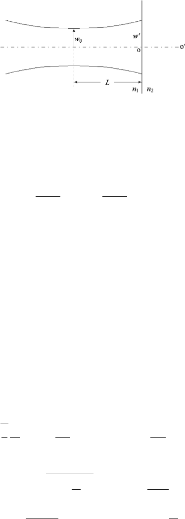
668 10. Scalar Diffraction Theory
Figure 10.24: Normal incidence of a Gaussian beam on the surface between
different media.
As the light propagates perpendicularly to the optical axis, that is α = π/2,
then
a
x
= 0, b
x
=
n
e
2k
0
n
2
o
, b
y
=
1
2k
0
n
e
, k
e
= (n
e
+ δn
e
)k
0
.
In principle, the propagation of electromagnetic waves in media with arbi-
trary index distribution can be treated with (10.207)–(10.211).
10.6.6 Reflection and Refraction of Gaussian Beams
on Medium Surfaces
In Section 10.5 we discussed the refraction of a Gaussian beam on the surface
of a crystal. Since we supposed that the radius of the beam waist was much
larger than the wavelength, the reflectance was uniform on the surface of
the medium. If the beam waist is not much larger than the wavelength, the
reflectance will vary on the surface, which must be taken into account in
deriving the reflected and refracted beams.
For simplicity, here we discuss only the case of normal incidence. In
Fig. 10.24, a Gaussian beam is normally incident on medium 2 from medium
1. The boundary between the media is at z = 0. The beam waist is located
at z = −L, and the radius of the waist is w
0
. The amplitude distribution of
the incident beam on the boundary is
ψ(ρ, 0) =
r
2
π
1
w
0
exp
µ
−
ρ
2
w
02
exp
·
−jk
1
µ
L +
ρ
2
2R
0
+ jφ
0
¸
, (10.212)
where
w
0
= w
0
s
1 +
µ
L
s
1
2
, s
1
=
k
1
w
2
0
2
,
R
0
=
L
2
+ s
2
1
L
, φ
0
= arctan
µ
L
s
1
.

10.6 Eigenwave Expansions of Electromagnetic Fields 669
In the above equations k
1
= 2n
1
π/λ, n
1
is the refractive index in medium
1. According to (10.177), the amplitude of the eigenmode in a cylindrical
coordinate system is
F (k
ρ
) =
Z
∞
0
ψ
0
(ρ
0
, 0)J
0
(k
ρ
ρ
0
)ρ
0
dρ
0
. (10.213)
By introducing (10.183), (10.185), and (10.186), the integration of (10.213)
is
F (k
ρ
) =
r
1
2π
w
0
exp
"
−
µ
k
ρ
w
0
2
2
#
exp
"
−jL
Ã
k
1
−
k
2
ρ
2k
1
!#
. (10.214)
The reflection coefficient of the eigenmode at the boundary can be derived
from the continuous condition at the boundary. It is
Γ =
q
k
2
1
− k
2
ρ
−
q
k
2
2
− k
2
ρ
q
k
2
1
− k
2
ρ
+
q
k
2
2
− k
2
ρ
≈
k
1
− k
2
k
1
+ k
2
Ã
1 +
k
2
ρ
k
1
k
2
!
, (10.215)
where k
1
= 2n
1
π/λ, k
2
= 2n
2
π/λ, and n
1
and n
2
are the refractive indices
of the media. The transmission coefficient is then
T =
2
q
k
2
1
− k
2
ρ
q
k
2
1
− k
2
ρ
+
q
k
2
2
− k
2
ρ
≈
2k
1
k
1
+ k
2
µ
1 +
k
1
− k
2
2k
2
1
k
2
k
2
ρ
. (10.216)
The amplitude distribution of the reflected beam is
ψ = e
jk
1
z
Z
∞
0
F (k
ρ
)Γ J
0
(k
ρ
ρ) exp
Ã
−jk
2
ρ
z
2k
1
!
k
ρ
dk
ρ
=
r
1
2π
k
1
− k
2
k
1
+ k
2
w
0
exp[−jk
1
(L − z)]
Z
∞
0
exp
"
−
µ
k
ρ
w
0
2
2
#
exp
µ
jk
2
ρ
L − z
2k
1
J
0
(k
ρ
ρ)
Ã
1 +
k
2
ρ
k
1
k
2
!
k
ρ
dk
ρ
=
r
2
π
k
1
− k
2
k
1
+ k
2
1
w
1
exp[−jk
1
(L − z)] exp
µ
−
ρ
2
w
2
1
exp
µ
−
jk
1
ρ
2
2R
1
+ jφ
1
·
1 +
4
k
1
k
2
w
1
w
0
exp(jφ
1
) −
4ρ
2
k
1
k
2
w
2
1
w
2
0
exp(2jφ
1
)
¸
, (10.217)
where
w
1
= w
0
s
1+
µ
L−z
s
2
, R
1
=
(L−z)
2
+s
2
L − z
, φ
1
= arctan
µ
L−z
s
.

670 10. Scalar Diffraction Theory
Equation (10.217) can also be expressed as
ψ = ψ
gs1
·
1 +
4
k
1
k
2
w
1
w
0
exp(jφ
1
) −
4ρ
2
k
1
k
2
w
2
1
w
2
0
exp(2jφ
1
)
¸
, (10.218)
where
ψ
gs1
=
r
2
π
k
1
− k2
k
1
+ k
2
1
w
1
exp[−jk
1
(L − z)] exp
µ
−
ρ
2
w
2
1
exp
µ
−
jk
1
ρ
2
2R
1
+ jφ
1
.
(10.219)
The reflected beam is distributed in the left half-space, so in (10.217)–(10.219)
z < 0. The distribution of the refracted beam is
ψ = e
−jk
2
z
Z
∞
0
F (k
ρ
)T J
0
(k
ρ
ρ) exp
Ã
jk
2
ρ
z
2k
2
!
k
ρ
dk
ρ
=
r
1
2π
2k
1
k
1
+ k
2
w
0
exp[−j(k
1
L + k
2
z)]
Z
∞
0
exp
"
jk
2
ρ
L
2k
1
+
jk
2
ρ
z
2k
2
−
µ
k
ρ
w
0
2
2
#
J
0
(k
ρ
ρ)
µ
1 +
k
1
− k
2
2k
2
1
k
2
k
2
ρ
k
ρ
dk
ρ
=
r
2
π
2k
1
k
1
+ k
2
1
w
2
exp[−j(k
2
z + k
1
L)] exp
µ
−
ρ
2
w
2
2
exp
µ
−
jk
2
ρ
2
2R
2
+ jφ
2
·
1 +
2(k
1
− k
2
)
k
2
1
k
2
w
2
w
0
exp(jφ
2
) −
2ρ
2
(k
1
− k
2
)
k
2
1
k
2
w
2
2
w
2
0
exp(2jφ
2
)
¸
, (10.220)
where
w
2
= w
0
s
1 +
1
s
2
2
µ
z +
k
2
k
1
L
2
, φ
2
= arctan
·
1
s
2
µ
z +
k
2
k
1
L
¶¸
,
R
2
=
µ
z +
k
2
k
1
L
2
+ s
2
2
z +
k
2
k
1
L
, s
2
=
k
2
w
2
0
2
.
Equation (10.220) can also be expressed as
ψ = ψ
gs2
·
1 +
2(k
1
− k
2
)
k
2
1
k
2
w
2
w
0
exp(jφ
2
) −
2ρ
2
(k
1
− k
2
)
k
2
1
k
2
w
2
2
w
2
0
exp(2jφ
2
)
¸
, (10.221)
where
ψ
gs2
=
r
2
π
2k
1
k
1
+ k
2
1
w
2
exp[−j(k
2
z + k
1
L)] exp
µ
−
ρ
2
w
2
2
exp
µ
−
jk
2
ρ
2
2R
2
+ jφ
2
.
(10.222)
From (10.220) and (10.221) we know that neither the reflected beam nor
the refracted b eam are standard Gaussian beams. If w
0
À λ, the non-
uniformity of the reflection on the dielectric boundary can be neglected, and
the reflected and the refracted beams are both standard Gaussian beams.