Baker K.R. Optimization Modeling with Spreadsheets

Подождите немного. Документ загружается.

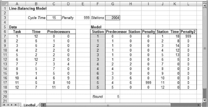
Figure 9.9 shows a spreadsheet model, with the given information reproduced in

columns A–D. The optimization model occupies columns F –L. Row 3 contains the

desired cycle time, a penalty, and the objective function. The penalty, shown in this

example as the value 999, must be a large number, adjusted to the scale of the data

in the problem.

The range F7:F18 contains the decision variables of the model. These are the

station numbers assigned to the tasks. These variables must be integers starting at 1

and increasing to the number of stations in the solution. Although we don’t know

that number in advance, we can make a conservative guess and use this guess as an

upper bound when we specify the problem. The solution in column F of Figure 9.9

arbitrarily assigns two tasks to each station, proceeding roughly in order of the

tasks. Columns G and H reference the predecessors in columns C and D and look

up their stations using the INDEX function. The two columns allocated to the prede-

cessor list in the given data (columns C and D) and the two columns allocated to the

predecessor-station list in the model (columns G and H) are used because no task in the

problem has more than two predecessors. Obviously, this layout would have to be

modiﬁed for problems with more than two predecessors for some tasks.

Column I contains a feasibility check to see whether each task is assigned a station

number at least as large as that of its predecessors. If not, the penalty from cell E2 is

assigned. In the solution of Figure 9.9, task 10 is assigned to station 6 and task 11 to

station 5. But task 10 is a predecessor to task 11, so those assignments are out of pre-

cedence order. Hence the penalty in cell I17.

Columns J, K, and L represent a table that examines the solution station by station.

(This table may actually not need the same number of rows as the rest of the model, but

extra rows can simply be assigned zeros.) Column K shows the total time assigned to

each station, using the SUMIF (see Box 9.2) function. Finally, column L contains

Figure 9.9. Spreadsheet model for Example 9.2.

356 Chapter 9 Heuristic Solutions with the Evolutionary Solver

another feasibility check and assigns a penalty to any station assigned a total time that

exceeds the desired cycle time in cell C3.

Finally, cell G3 is the objective function. It contains the maximum value among

the decision variables (the assigned station numbers), augmented by the total of the

penalties. The use of penalties thus substitutes for explicit feasibility constraints.

The only constraints that need to be speciﬁed for Solver are the upper and lower

limits on the station assignments. As mentioned earlier, the lower limit is obviously

one, but the upper limit requires an educated guess. In the worst case, each task

would be assigned its own station, so we can always use the number of tasks as an

upper limit. We specify the problem as follows.

Objective: G3 (minimize)

Variables: F7:F18

Constraints: F7:F18  12

F7:F18  1

F7:F18 ¼ integer

One last step is helpful in the line-balancing model. As we use the evolutionary

solver to search among solutions, it is helpful to know a lower bound on the minimum

possible number of stations. This lower bound can be calculated by taking the sum of

the task times, dividing by the desired cycle time, and rounding up to the next larger

BOX 9.2

Excel Mini-Lesson: The SUMIF Function

The familiar SUM function in Excel computes the total value in the cells of a speciﬁed

range. The SUMIF function is similar, in that it totals the values in a range of cells

(called the sum range), but it includes only those items in the range for which a speciﬁed

criterion is met. To satisfy the criterion, a speciﬁed condition must be met in a speciﬁed

range. The form of the function is the following.

¼ SUMIF(Specified range, Criterion, Sum range)

In Example 9.2, we have

Speciﬁed range: F7:F18 (the list of station assignments)

Criterion: a reference to a cell in column J (that is, a station number)

Sum range: B7:B18 (the list of task times).

Thus, in cell K10 we have the formula

¼ SUMIF($F$7:$F$18 ,J10,$B$7:$B$18).

This function scans the list in column F to see if any entries match the contents of cell

J10 (which is station number 4), and if so, the corresponding entry in column B is included

in the sum. When the entire list has been scanned, the function returns the sum of the task

times assigned to station 4, which in this case is 12.

9.6. Line Balancing

357

integer. This bound follows from the observation that if the tasks were packed into

stations with perfect efﬁciency, the sum of the task times at each station would

equal the desired cycle time, and the total sum of the task times divided by the

cycle time would give the number of stations. In Example 9.2, the sum of the task

times divided by the desired cycle time yields the value 4.67, which rounds up to 5.

This calculation appears in cell G20. It allows us to stop searching if we see that

the evolutionary solver has located a solution with this value. However, it is important

to keep in mind that the lower bound may not be achievable; the optimal solution may

lie above the lower bound, so we will not always be able to tell whether our searching

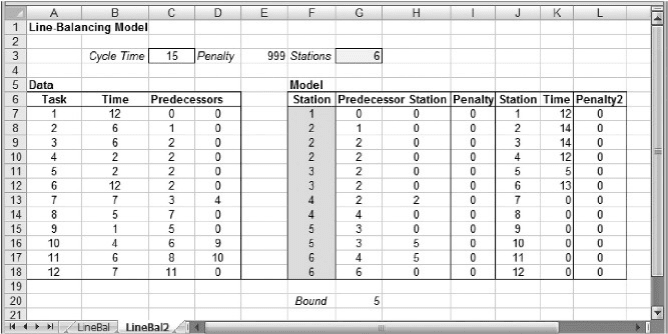
should be terminated. In Example 9.2, the evolutionary solver leads us repeatedly to a

solution with 6 stations, but we cannot be sure whether an improvement to ﬁve is poss-

ible. Figure 9.10 shows one of those solutions. In this solution, task 1 alone is assigned

to station 1; tasks 2–4 are assigned to station 2; and then tasks are assigned in numeri-

cal order, two to a station. From this solution, however, we cannot know whether a

ﬁve-station solution exists, but Munoz still has a reasonably efﬁcient set of station

assignments for its assembly line.

9.7. GROUP ASSIGNMENT

In several different application areas, a common problem involves the organization

of items or people into groups. Often, the goal is to place similar items in the same

group, as in cellular manufacturing (where we try to group similar parts together)

or in positioning analysis (where we try to group similar products together).

Sometimes, the goal is the opposite: to place different items in the same group. A fam-

iliar example in educational programs involves the formation of diverse student teams

(where we try to form groups of students with dissimilar backgrounds for the purposes

Figure 9.10. Final solution for Example 9.2.

358 Chapter 9 Heuristic Solutions with the Evolutionary Solver

of carrying out a particular group task). Business applications of the same type of

model arise when consultants are assigned to different project teams or trainees are

assigned to discussion groups. An example of forming student groups arises in a

typical course project.

EXAMPLE 9.3

Oxbridge College’s Accounting Department

Each term, the Accounting Department at Oxbridge assigns students to teams for the purposes of

a simulated audit engagement. In this problem, we are given a description of each student on

various dimensions, expressed with a set of zeros and ones. In particular, the Department has

recorded the following information for each student.

†

Majored in accounting as an undergraduate (1 ¼ yes, 0 ¼ no).

†

Previously worked for an accounting ﬁrm (1 ¼ yes, 0 ¼ no).

†

Gender (1¼ male, 0 ¼ female).

†

International background (1 ¼ yes, 0 ¼ no).

This term, 20 students will be participating in the exercise, and there will be ﬁve 4-person

teams. For the purposes of this exercise, the Department’s goal is to achieve diversity in its

assignment of students to teams.

In Example 9.3, each student is described by a string of four binary digits. For

example, a male student from the US who had not majored in accounting but

had worked for an accounting ﬁrm would be represented by the string {0, 1, 1, 0}.

A natural deﬁnition of decision variables for this problem is the following

¼ 1 if student j is assigned to group k, and 0 otherwise.

Suppose now that we want to form ﬁve teams of four students each. We can

express the essential constraints in the problem as follows

¼ 4 for k ¼ 1to5

¼ 1 for j ¼ 1to20

The ﬁrst set of these constraints ﬁxes the size of each group; the second set ensures

that each student is assigned to a unique group. If we model the decisions this way,

the problem contains 25 constraints and 100 variables. This is too large a pair of

numbers to expect the evolutionary solver to perform effectively.

The usual approach to an objective function builds on a metric that, for each attri-

bute, calculates the sum of squared differences from the population average. Suppose,

for example, that there are 10 accounting majors in the group of 20. Then the average

number per group is two. Suppose that the number of accounting majors assigned to

9.7. Group Assignment 359

the respective groups follows the proﬁle {1, 2, 2, 3, 2}. Then the calculation of the

performance measure is as follows.

(1  2)

þ (2  2)

þ (3  2)

þ (2  2)

¼ 2

If the proﬁle is {1, 0, 2, 3, 4}, then the metric is 10. Clearly, the ideal distribution

of accounting majors among the groups would generate a metric of zero. For an objec-

tive function, we usually calculate the metric for each attribute and then sum over the

attributes. This objective function can thus be expressed as a nonlinear function of the

decision variables x

Although this is a natural formulation of the problem, it creates difﬁculties for two

types of solution approaches. First, a direct formulation as an optimization problem

leads to a nonlinear programming model with integer variables. As we pointed out

in Chapter 8, this class of problems is poorly suited to the nonlinear solver. Instead,

it makes sense to tackle the problem with the evolutionary solver. However, the natural

formulation is also poorly suited to the evolutionary solver because it has many con-

straints and variables.

An alternative formulation of the problem can take advantage of the alldifferent

constraint. Here, we let

¼ student number assigned to position i

where there are 20 positions: four corresponding to the ﬁrst group, four for the second

group, and so on. The assignment of students to positions is equivalent to an assign-

ment of students to groups. In our example, the y

values need to satisfy the alldifferent

constraint for the integers from 1 to 20. From that deﬁnition, we can build a spread-

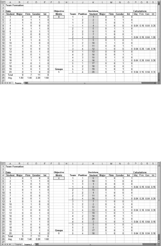
sheet model well suited to the evolutionary solver. Figure 9.11 shows the model.

The problem data occupy columns A – E, with a four-element string for each student.

The solution is described in columns I–K, where the shaded decision cells give the

assignment of student numbers to groups and positions. The squared differences

between each group’s attribute count and the population mean are calculated in col-

umns P–S, and their sum appears in cell G5 as the objective function. Although

this may seem to be a complicated way of computing the objective, it is nevertheless

suitable for the evolutionary solver.

We specify the problem as follows.

Objective: G5 (minimize)

Variables: K5:K24

Constraints: K5:K24 ¼ alldifferent

Again, the alldifferent constraint is sufﬁcient to capture the constraints of the model.

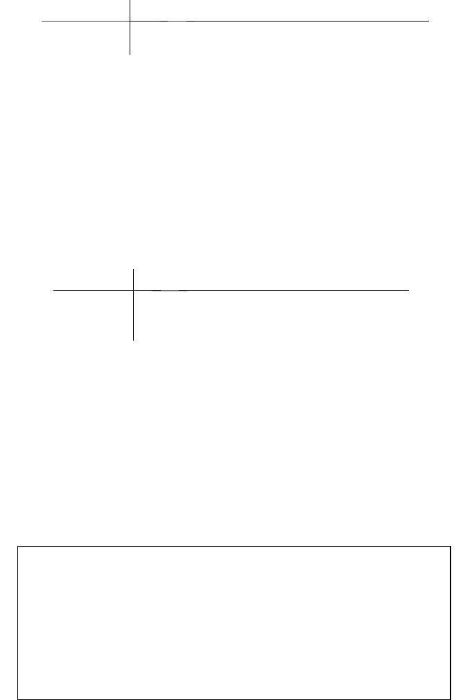
Starting with different assignments, the evolutionary solver takes us in most cases to a

solution with a metric of 4 quite quickly (see Figure 9.12), suggesting, perhaps, that

this is likely to be the optimal value. Alternative starting points and modiﬁcations

of the options do not seem to produce any improvement. Again, this is stronger evi-

dence that we might have found the optimum, although the evidence is not conclusive.

360

Chapter 9 Heuristic Solutions with the Evolutionary Solver

By using the evolutionary solver, administrators at the Accounting Department can

achieve their assignment goals where other methods, such as nonlinear integer pro-

gramming, would likely have failed.

The group assignment problem illustrates the fact that there may be creative

ways of formulating models to take advantage of the alldifferent constraint.

This means that we may want to think beyond the typical structures of linear and

nonlinear programming models, but no standard templates have been developed in

this regard.

Figure 9.12. Final solution for Example 9.3.

Figure 9.11. Spreadsheet model for Example 9.3.

9.7. Group Assignment 361

SUMMARY

The evolutionary solver contains an algorithm that complements the linear solver, the nonlinear

solver, and the branch-and-bound procedure. Unlike those algorithms, however, it does not

explicitly seek a local optimum or a global optimum. Nevertheless, it can often ﬁnd optimal sol-

utions to very difﬁcult problems, and it may be the only effective procedure we can apply when a

nonsmooth function exists in the model.

The considerations inﬂuencing the building of models for the evolutionary solver are

different from those for linear and nonlinear programs. Because nonsmooth functions are per-

mitted, we have great ﬂexibility in drawing on Excel’s various built-in functions if we wish to

calculate complex results in convenient ways. Also, experience suggests that the evolutionary

solver performs best if the number of variables and the number of constraints is not large. To

avoid constraints, we can often impose a numerical penalty when a condition is violated and

include the penalty in the objective function instead of entering the constraint explicitly.

Having built a model this way, it is helpful if we can start with an initial solution that satisﬁes

all constraints—that is, a solution without penalties. Otherwise, the evolutionary solver may not

be effective at ﬁnding feasible solutions (those without penalties) in models that contain penalty

terms in the objective.

The evolutionary solver is not likely to be trapped by local optima, as is the case with the

nonlinear solver. This feature is advantageous in searching for good solutions to problems con-

taining nonsmooth functions, especially nonlinear problems with integer variables. On the other

hand, we must realize that the search procedure is both random (subject to probabilistic vari-

ation) and heuristic (not guaranteed to ﬁnd an optimum). For that reason, we usually reserve

the use of the evolutionary solver for only the most difﬁcult problems.

The evolutionary solver works with a set of specialized parameters. Although we offered

default settings, these settings are merely a starting point. Different choices might be suitable

for different problem types. In addition, we may want to use one set of choices at the start

and then other settings in subsequent runs, while we look for improvements. As compared

to arbitrary settings, the intelligent selection of these parameters can enhance the performance

of the evolutionary solver considerably. Aside from the guidelines given here, practice

and experience using the evolutionary solver are the key ingredients in effective parameter

selection.

EXERCISES

9.1. Sequencing Jobs A fundamental model in scheduling contains a set of jobs that are

waiting to be processed by a machine or processor. The machine is capable of handling

only one job at a time, so the jobs must be processed in sequence. The problem is to ﬁnd

the best sequence for a given objective function.

For example, the processor might be an integrated machining center that performs a

number of metal-cutting operations on components for complex assemblies. Ten different

components have reached the center and are awaiting processing. These jobs and their

processing times (expressed in hours) are described in the following table. In addition,

each job has a corresponding due date that has been calculated by the production control

system. As a result of the sequence chosen, each job will either be on time or late. If it is

late, the amount of time by which it misses its due date is called its tardiness. The objec-

tive is to minimize the total tardiness in the schedule.

362 Chapter 9 Heuristic Solutions with the Evolutionary Solver

Job 123 4 567 8910

Processing time 6 1 2 5 9 8 12 3 9 7

Due date 17 5 25 15 20 8 44 24 50 20

What is the minimum total tardiness and the sequence that achieves it?

9.2. Scheduling a Shop Midwest Parts Supply (MPS) is a fabricator of small steel parts

that are sold as components to manufacturers of electronic appliances and medical equip-

ment. In the MPS fabrication department, steel sheets are subjected to a series of three

main operations—cutting, trimming, and polishing. Each job must have the operations

completed in this order, and each machine sees the same job order, so it is sufﬁcient to

specify a single job sequence in order to describe a schedule. No machine can process

more than one job at a time.

This morning, 10 jobs have been released to the shop by the ERP system, and the

production manager is interested in minimizing the time it takes to complete the entire

schedule, usually referred to as the schedule makespan. The following table gives the

number of hours required for each operation.

Job 12345678910

Cutting time 1 5 3 7 9 7 8 8 3 6

Trimming time 2 9 2 10 7 6 9 9 1 1

Polishing time 9 7 3 4 7 8 9 4 1 3

What sequence achieves the minimum makespan and what is the minimum length of a

schedule?

9.3. Planning a Tour Recent graduate and amateur world traveler Alastair Bor is planning

a European trip. His preferences are inﬂuenced by his curiosity about urban culture in

Europe and by his extensive study of international relations while he was in school.

Accordingly, he has decided to make one stop in each of 12 European capitals in

the time he has available. He wants to ﬁnd a sequence of the cities that involves the

least total mileage. He has calculated inter-city distances using published data on latitude

and longitude, and applying the geometry for arcs of great circles. These distances are

shown below.

Ams. Ath. Ber. Brus. Cope. Dub. Lis. Lon. Lux. Mad. Par. Rom.

From

Amsterdam – 2166 577 175 622 712 1889 339 319 1462 430 1297

Athens 2166 – 1806 2092 2132 2817 2899 2377 1905 2313 2100 1053

Berlin 577 1806 – 653 348 1273 2345 912 598 1836 878 1184

Brussels 175 2092 653 – 768 732 1738 300 190 1293 262 1173

Copenhagen 622 2132 348 768 – 1203 2505 942 797 2046 1027 1527

Dublin 712 2817 1273 732 1203 – 1656 440 914 1452 743 1849

Lisbon 1889 2899 2345 1738 2505 1656 – 1616 1747 600 1482 1907

London 339 2377 912 300 942 440 1616 – 475 1259 331 1419

Luxembourg 319 1905 598 190 797 914 1747 475 – 1254 293 987

Madrid 1462 2313 1836 1293 2046 1452 600 1259 1254 – 1033 1308

Paris 430 2100 78 262 1027 743 1482 331 293 1033 – 1108

Rome 1297 1053 1184 1173 1527 1849 1907 1419 987 1308 1108 –

What sequence achieves a minimum-distance tour for Alastair, starting in Brussels,

and what is the minimum tour length?

Exercises 363

9.4. Cutting Stock Poly Products sells packaging tape to industrial customers. All tape is

sold in 100-foot rolls that are cut in various widths from a master roll, which is 15

inches wide. The product line consists of the following widths: 2

, and 11

These can be cut in different combinations from a 15-inch master roll. For example,

one combination might consist of three cuts of 5

each. Another combination might con-

sist of two 2

cuts and an 11

cut. Both of these combinations use the entire 15-inch roll

without any waste, but other combinations are also possible. For example, another com-

bination might consist of two 7

cuts. This combination creates one inch of waste for

every roll cut this way.

Each week, Poly Products collects demands from its customers and distributors

and must ﬁgure out how to conﬁgure the cuts in its master rolls. To do so, the production

manager lists all possible combinations of cuts and tries to ﬁt them together so that waste

is minimized while demand is met. (In particular, demand must be met exactly, because

Poly Products does not keep inventories of its tape.) This week’s demands are shown

in the table.

Size 2

Demand 60 50 40 30 20

(a) How many combinations can be cut from a 15-inch master roll so that there is less

than two inches of waste (i.e. the smallest quantity that can be sold) left on the roll?

(b) Find a set of combinations that meets demand exactly and generates the minimum

amount of waste. (Stated another way, the requirement is to meet or exceed

demand for each size, but any excess must be counted as waste.) What is the optimal

set of combinations and the minimum amount of waste?

9.5. Locating Warehouses Southeastern Foods has hired you to analyze their distribution

system design. The company has 11 distribution centers, with monthly volumes as

listed below. Seven of these sites can support warehouses, in terms of the infrastructure

available, and are designated by (W).

Center Volume Center Volume

Atlanta (W) 5000 Memphis (W) 7800

Birmingham (W) 3000 Miami 4400

Columbia (W) 1400 Nashville (W) 6800

Jackson 2200 New Orleans 5800

Jacksonville 8800 Orlando (W) 2200

Louisville (W) 3000

The monthly ﬁxed cost for operating one of these warehouses is estimated at

$3600, although there is no capacity limit in their design. Southeastern could build ware-

houses at any of the designated locations, but its criterion is to minimize the total of

ﬁxed operating costs and variable shipment costs. Information has been compiled show-

ing the cost per carton of shipping from any potential warehouse location to any distri-

bution center.

364 Chapter 9 Heuristic Solutions with the Evolutionary Solver

Atl Bir Col Jac Jvl Lvl Mem Mia Nash NewO Orl

Atlanta 0.00 0.15 0.21 0.40 0.31 0.42 0.38 0.66 0.25 0.48 0.43

Birmingham 0.15 0.00 0.36 0.25 0.46 0.36 0.26 0.75 0.19 0.35 0.55

Columbia 0.21 0.36 0.00 0.60 0.30 0.50 0.62 0.64 0.44 0.69 0.44

Louisville 0.42 0.36 0.50 0.59 0.73 0.00 0.38 1.09 0.17 0.70 0.86

Memphis 0.38 0.26 0.62 0.21 0.69 0.38 0.00 1.00 0.21 0.41 0.78

Nashville 0.25 0.19 0.44 0.41 0.56 0.17 0.21 0.91 0.00 0.53 0.69

Orlando 0.43 0.55 0.44 0.70 0.14 0.86 0.78 0.23 0.69 0.65 0.00

(a) What is the minimum total cost?

(b) To achieve the cost in (a), which warehouse locations should be used?

9.6. Locating Emergency Centers After the damage caused in Florida by a series of

severe hurricanes, the governor ordered the Florida Emergency Management Agency

(FLEMA) to design a systematic plan for emergency services following severe

weather events. The state has 11 emergency ofﬁces, and it would be possible to build a

warehouse next to each of the ofﬁces to store emergency equipment. As a consultant to

FLEMA, you were asked to determine how many centers would be needed to ensure

that there would be a warehouse within 50 miles of any emergency ofﬁce. After studying

your recommendation, however, FLEMA’s Director decided that the cost of the plan

would be prohibitive, so a revised formulation was developed. This one requires building

just four warehouses.

With this standard in mind, you have obtained the distances between the eleven

ofﬁces (identiﬁed by their cities).

DB Ft L Ft M Gain Mia Nap Orl St P Sara Talla Tam

Daytona

Beach

0 229 207 98 251 241 54 159 186 234 139

Ft Lauderdale 229 0 133 312 22 105 209 234 202 444 234

Ft Myers 207 133 0 230 141 34 153 110 71 356 123

Gainesville 98 312 230 0 331 264 109 143 179 144 128

Miami 251 22 141 331 0 107 228 251 214 463 245

Naples 241 105 34 264 107 0 187 143 107 389 156

Orlando 54 209 153 109 228 187 0 105 132 242 85

St Petersburg 159 234 110 143 251 143 105 0 39 250 20

Sarasota 186 202 71 179 214 107 132 39 0 286 53

Tallahassee 234 444 356 144 463 389 242 250 286 0 239

Tampa 139 234 123 128 245 156 85 20 53 239 0

FLEMA would like to ensure that there will be a warehouse center within x miles of any

ofﬁce. What is the minimum value of x that can be achieved when there are four ware-

houses in the system?

9.7. Touring the Agents Professor Moonlight runs a fund of funds in order to supplement

his academic salary. Every winter, he pays a visit to each of the fund managers with whom

he works. These visits are all made in one trip, during which he visits investment agents in

nine cities. Prof. Moonlight doesn’t mind ﬂying, but he dislikes long ﬂights. For this trip,

he wants to ﬁnd a route through the various cities starting and ending in San Antonio, and

he wants the longest leg of the trip (measured in miles) to be as short as possible. The pair-

wise distances in miles are shown below.

Exercises 365