Baker K.R. Optimization Modeling with Spreadsheets

Подождите немного. Документ загружается.

for 64-bit Risk Solver Platform, named RSPSetup64.exe. In all other cases, you’ll

download and run RSPSetup.exe. Running the Setup program is straightforward,

but you’ll need to pay attention to three prompts.

1. You’ll be asked for an installation password. This will be emailed to you, at the

email address you give when you ﬁll out the registration form.

2. You’ll be asked for a license activation code. This appears in the same email as

the installation password; it determines whether you’ll be using full RSP for 15

days, RSPE for 140 days, or something else.

3. You’ll be asked whether you want to run initially as full Risk Solver Platform,

or a subset product. There are several choices, but for use with this book, the

recommended selection is Premium Solver Platform. (You can change this

selection later, using Help—About on the RSP/PSP Ribbon.)

To uninstall the software, you can either re-run RSPSetup.exe, or use the Windows

Add/Remove Programs feature.

A1.2. SUPPLEMENTAL EXCEL FILES

This book is supported by a website that contains supplementary ﬁles. The URL for

the website is http://mba.tuck.dartmouth.edu/opt/. Speciﬁcally, the website contains

a collection of Excel ﬁles corresponding to all of the spreadsheet exhibits in the book.

This collection is not intended merely for backup purposes: you are encouraged to

open these ﬁles while reading the text and to explore them carefully. This exploration

provides a hands-on feel for the examples in the text and potentially serves as a tem-

plate for other, similar problems.

A second collection of Excel ﬁles contains data sets for selected end-of-chapter

exercises and cases. The data sets are provided for situations in which it would be

tedious to enter all the data into an Excel ﬁle for the purpose of working on the

exercise.

Some of the cases contain references to an existing spreadsheet model. The web-

site also contains Excel ﬁles for these models.

376

Appendix 1 Optimization Software and Supplemental Files

Appendix 2

Graphical Methods in Linear

Programming

We can use graphical methods to solve linear optimization problems involving two

variables. When there are two variables in the problem, we can refer to them as x

and x

, and we can do most of the analysis on a two-dimensional graph. Although

the graphical approach does not generalize to a large number of variables, the basic

concepts of linear programming can all be demonstrated in the two-variable context.

When we run into questions about more complicated problems, we can ask, what

would this mean for the two-variable problem? Then, we can look for answers in

the two-variable case, using graphs.

Another advantage of the graphical approach is its visual nature. Graphical

methods provide us with a picture to go with the algebra of linear programming,

and the picture can anchor our understanding of basic deﬁnitions and possibilities.

For these reasons, the graphical approach provides useful background for working

with linear programming concepts.

A2.1. AN EXAMPLE

Consider the planning and scheduling problem facing a manufacturer of microwave

ovens with two models in its line—the standard and the deluxe. Each oven is

assembled from component parts and subassemblies that are produced in the mechan-

ical and electronics departments. The following table shows the number of production

hours per oven required in each department and the capacities of the three production

departments, in monthly hours.

Standard (h/oven) Deluxe (h/oven) Capacity (h/mo)

Assembly Department 4 4 560

Mechanical Department 3 2 400

Electronics Department 2 4 400

Optimization Modeling with Spreadsheets, Second Edition. Kenneth R. Baker

# 2011 John Wiley & Sons, Inc. Published 2011 by John Wiley & Sons, Inc.

377

The sales department believes that there will be demand for as many ovens as the

company can produce. The accounting department has determined that the variable

proﬁt contributions are $50 for each standard and $40 for each deluxe. The problem

is to determine a production plan to maximize monthly proﬁt contribution.

Our ﬁrst step in analyzing this problem is to express it algebraically. The problem

of devising an output plan boils down to ﬁnding the best number of standard ovens and

deluxe ovens for the ﬁrm to produce in the coming month. Thus, we let

¼ number of standard ovens

¼ number of deluxe ovens

Once we determine the values of x

and x

, the problem will be solved. Furthermore,

the criterion is to maximize the proﬁt contribution generated by our plan. In particular,

we can write our objective function as

Maximize z ¼ 50x

þ 40x

where z represents the value of the objective function.

Having speciﬁed decision variables and an objective function, we turn our atten-

tion to the constraints of the problem, the limited capacities in the assembly, mechan-

ical, and electronics departments. In assembly, the number of hours consumed by a

production schedule cannot exceed the 560 hours available. We can write this require-

ment algebraically as

þ 4x

 560

Similarly, for the mechanical and electronics departments, we require

þ 2x

 400

þ 4x

 400

In standard form, an algebraic statement of our full model is

Maximize z ¼ 50x

þ 40x

subject to 4x

þ 4x

 560 (A)

þ 2x

 400 (M)

þ 4x

 400 (E)

Finally, implicit in our deﬁnition of the two decision variables is the requirement that

they must both remain nonnegative (x

 0 and x

 0).

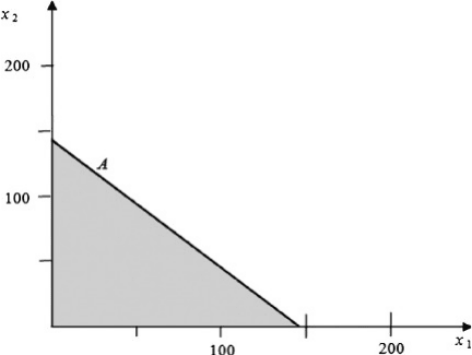
We begin the graphical analysis with the constraints. For a graphical approach, we

can work with equations more readily than inequalities, so we consider the equations

corresponding to each of the constraints in turn. For the assembly department con-

straint (A), the line 4x

þ 4x

¼ 560 deﬁnes the locus of all points at which the depart-

ment is fully utilized. That is, the line represents the set of product mix combinations

378

Appendix 2 Graphical Methods in Linear Programming

, x

) that consume all 560 available hours in assembly. To plot the line, note that the

intercept is 140 (obtained by setting x

¼ 0 and solving the equation for x

Similarly, the x

intercept is 140. Plotting the two intercepts, (140, 0) and (0, 140)

on a graph, and connecting the two points with a straight line, we construct the plot

shown in Figure A2.1, where the label A on the graph is used to associate this line

with the assembly hours constraint.

The line plotted in Figure A2.1 represents all combinations (x

, x

) that consume

exactly 560 hours of assembly time. Our model, however, looks for combinations that

consume no more than 560 hours. Combinations that consume fewer that 560 hours

are also admissible, and these correspond to points (x

, x

) that lie below the line.

In fact, if we consider only the points that are admissible in the assembly constraint

and that also meet the nonnegativity requirements, then we are left with the shaded

triangle shown in Figure A2.1.

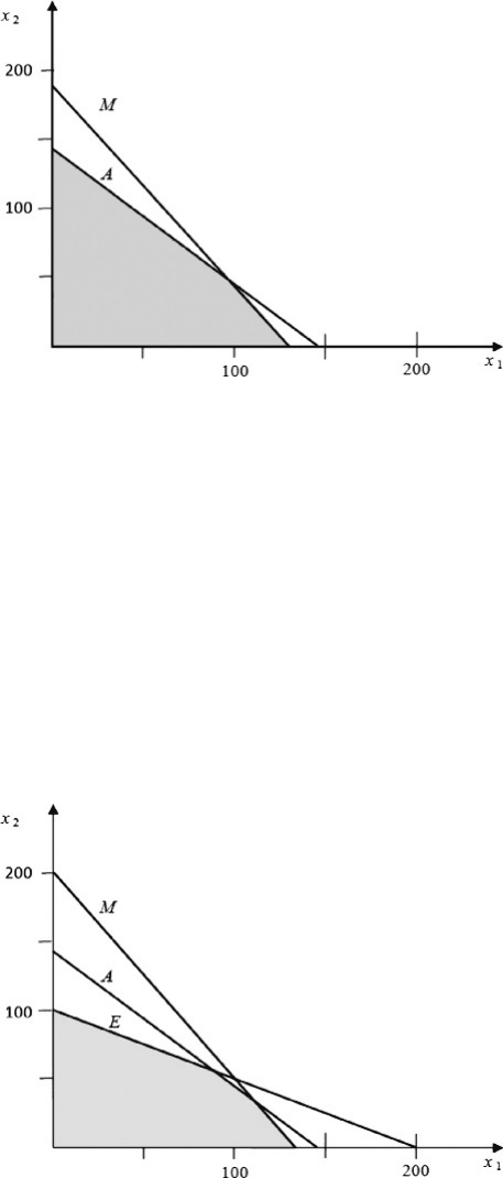
Next, we plot a line corresponding to mechanical department hours, or 3x

¼ 400, as shown in Figure A2.2 with the label M. Points on this line represent

combinations of standard and deluxe ovens that consume exactly 400 hours of mech-

anical time, and points below the line consume fewer than 400 hours. The line corre-

sponding to the mechanical department has a slope of – 3/2, in comparison to the

assembly department line, which has a slope of –1. Only points that lie below both

constraint lines (and in the nonnegative region) are admissible decisions, as indicated

by the shading.

Finally, we plot a line corresponding to the electronic department limit, 2x

¼ 400, shown in Figure A2.3 with the label E. This line has a slope of –1/2,

and again we shade the region that lies below all three of the lines, as shown in

ﬁgure. The shaded region now represents the set of all points that are admissible

decisions: They satisfy all of the constraints in our problem.

The shaded area in Figure A2.3 is called the feasible region. It is a ﬁve-sided poly-

gon containing, along its boundary or inside, all of the points that correspond to

Figure A2.1. Sketch of ﬁrst

constraint.

A2.1. An Example 379

feasible decisions in our model. Our next step is to ﬁnd the best value of the objective

function that can be achieved by a point in this feasible region.

To pursue this search, consider what happens when we set the objective function

(z) equal to a ﬁxed value. For example, suppose z ¼ 2000. Then all points (x

, x

) that

achieve a value of 2000 in the objective function lie on the line 50x

þ 40x

¼ 2000.

Furthermore, all points that achieve a value of 2000 and that are feasible in the con-

straints lie along this line and within the feasible region. Consider a second line cor-

responding to z ¼ 4000. Like the ﬁrst objective function line, this one has a slope of

–5/4, so it is parallel to the ﬁrst. However, it has different intercepts and lies above and

to the right of the ﬁrst line, as shown in Figure A2.4. From these two lines, we can

imagine an entire family of lines, each with a slope of – 5/4 and each corresponding

Figure A2.2. Sketch of

second constraint.

Figure A2.3. Sketch of

third constraint.

380 Appendix 2 Graphical Methods in Linear Programming

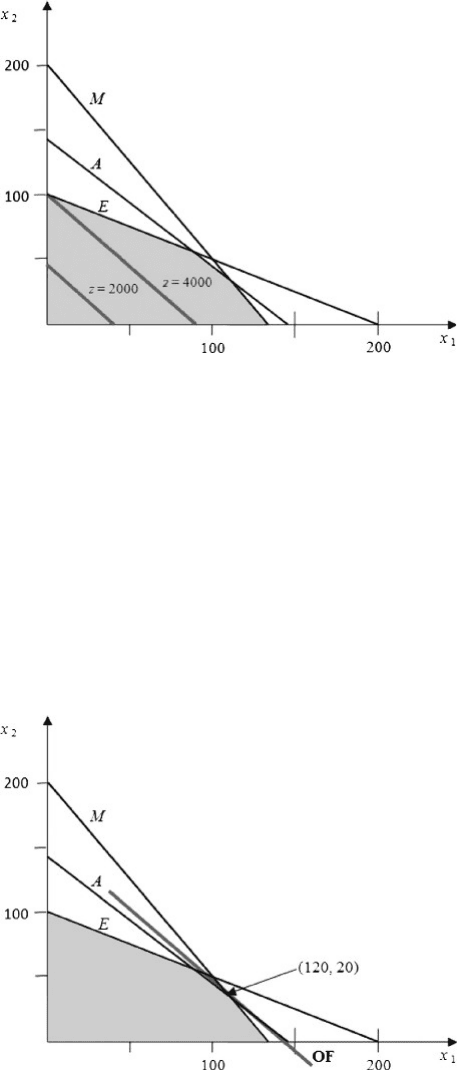
to a particular value of z. Relatively larger values of z correspond to lines in this family

that lie farther above and to the right. We wish to ﬁnd the largest value of z attainable in

this family and within the feasible region. A look at the ﬁgure indicates that this value

occurs at the intersection of the assembly and mechanical constraints.

We can make this result more precise by solving for the point at which the

assembly and mechanical constraints intersect. This point is (120, 20), as shown in

Figure A2.5, corresponding to a product mix of 120 standard ovens and 20 deluxe

ovens. The corresponding proﬁt total is $6800, corresponding to the objective function

line for z ¼ 6800, labeled OF in the ﬁgure. Using graphical methods, we have found

the best value of the objective function and the decisions that generate it.

Figure A2.4. Sketch of

objective function lines.

Figure A2.5. Sketch of

optimal point.

A2.1. An Example 381

A2.2. GENERALITIES

The oven-manufacturing problem was merely an example, but it does illustrate the

principles of graphical solution methods for optimization. In the example, all con-

straints are of the LT (less-than) variety. This means that points on the graph are feas-

ible if they lie on or below the corresponding constraint line. On the other hand, had we

encountered GT (greater-than) constraints, the feasible points would have been found

on or above the corresponding constraint line. The other possibil ity, EQ (equal-to)

constraints, would force us to consider only points lying directly on the constraint line.

In our example, the criterion was to maximize the objective function. By sketch-

ing the implications for two lines, each corresponding to a particular value of the

objective function (sometimes called an iso-value line), we can begin to see a

family of related objective function lines, leading to a maximum feasible value at

one corner of the feasible region. Our objective function contained all positive coefﬁ-

cients, so the process of maximization led us to lines ever higher and to the right on our

graph. Had we been interested in minimization (of a function with all positive coefﬁ-

cients), we would have been led to lines lower and to the left of a given starting point.

For other combinations involving negative coefﬁcients, the idea is to plot the graph of

two or three iso-value lines, in order to see where on the graph the optimum will ulti-

mately be found.

An examination of iso-value lines could reveal that there is no limit, in some

direction, to the value of the objective function. This would be the case if we were ana-

lyzing an unbounded problem. In other circumstances, attempting to delineate the

feasible region itself will reveal an infeasible problem, in which the constraints are

mutually contradictory. These two exceptional cases can therefore be identiﬁed

while carrying out the graphical analysis.

The graphical method is valuable because it produces a picture of the optimization

process. That picture may make it easier to interpret what occurs during an optimiz-

ation procedure. However, the graphical method is more difﬁcult when there are

three dimensions and impossible when there are more than three dimensions, so we

can use it only for relatively simple cases. Nevertheless, two-dimensional examples

illustrate most of the principles of linear programming.

As an example, suppose we consider well-posed linear programs in which the

feasible region exists and in which the objective function is not unbounded. The

theory tells us that an optimum can be found at one of the corners of the feasible

region. This property is very useful, because it means that we don’t have to search

for an optimal point in the interior of the region (an area that contains an inﬁnite

number of points.) Instead, we can limit our search to the boundary, and just to the

corner points on that boundary, which are ﬁnite in number. This is what most linear

programming codes do: They search systematically among the corner points on the

boundary of the feasible region, stopping only when an optimum has been located.

A second theoretical result tells us that we can identify an optimal corner point by

showing that its objective function value is better than those of its neighboring corner

points. Each of the corner points in our graph has two neighbors, and either of these

can be reached by moving along one of the boundaries of the feasible region. When we

382

Appendix 2 Graphical Methods in Linear Programming

start our search at one of the corner points, only two things can happen. Either the

objective function is better than at both neighboring corners (in which case, we

have found the optimum), or one of the neighbors has a better value. In the latter

case, we move to that point and then evaluate the neighboring possibilities from the

new location. In linear programming problems, we are essentially guaranteed that

this search procedure ultimately leads to the optimum. Indeed, this approach lies at

the heart of the simplex algorithm, which is the most popular method in use today

for ﬁnding solutions to linear programming problems. (For an algebraic glimpse of

the simplex method, see Appendix 3.)

A2.2. Generalities 383

Appendix 3

The Simplex Method

The simplex method is the algorithm most frequently used in computer programs for

solving linear programming problems. The linear solver in Excel is an implementation

of the simplex method, and the simplex method constitutes part of virtually every

successful commercial software package for optimization. In this appendix, we use

an example to illustrate the simplex method, and we comment on how the algorithm

can be adapted to special situations that arise.

A3.1. AN EXAMPLE

We use a variation of Example 2.1 to illustrate how the simplex method works. For this

purpose, we drop the wo od constraint and address the following optimization problem.

Maximize z ¼ 16C þ20D þ14T

subject to

4C þ6D þ2T  2000

3C þ8D þ6T  2000

9C þ6D þ4T  1440

The simplex method works not with inequalities but rather with equalities, so our ﬁrst

step is to recast the constraints of the model as equations. To do so, we introduce three

additional variables that account for unused amounts of the three resources. In other

words, these variables represent the difference between the right-hand side (RHS)

and left-hand side (LHS) of the constraints, as they are posed above. The constraints

may be written as follows.

Set 1 : 4C þ 6D þ 2T þu ¼ 2000 (A3:1)

3C þ 8D þ 6T þv ¼ 2000 (A3: 2)

9C þ 6D þ 4T þw ¼ 1440 (A3:3)

The variables u, v, and w are called slack variables: they measure the amount of slack,

or unused resource, in each constraint. These three variables, like the three original

Optimization Modeling with Spreadsheets, Second Edition. Kenneth R. Baker

# 2011 John Wiley & Sons, Inc. Published 2011 by John Wiley & Sons, Inc.

385