Baker R.C. Flow Measurement Handbook: Industrial Designs, Operating Principles, Performance, and Applications

Подождите немного. Документ загружается.

9.2 PRINCIPAL DESIGNS OF LIQUID METERS 187

loss is 0.5-1 bar, and pressure may be up to 40 bar or higher for certain designs, with

temperature up to 290°C.

Transmission may be through a permanent magnet coupling or through magnets

embedded in the oval wheels that generate a voltage in an external inductive sensor.

Calibration gearing may also pass the output to a totalizing counter. Operation may

be bidirectional.

Materials may be, for the body, stainless steel, cast iron, or aluminum and, for

the gears, carbon steel, brass, or chemical-resistant plastic.

Applications are in adhesives and polymers, but also in many basic utility flows

in the water industry and in hydraulic test stands. One manufacturer includes

solvents, paints, and adhesives; dispersions, polymerisates, and polycondensates;

glucose and alcohols; organic and inorganic liquids; gasoline, fuel oils, lubricants,

and raw and intermediate liquid products; and other liquid chemicals.

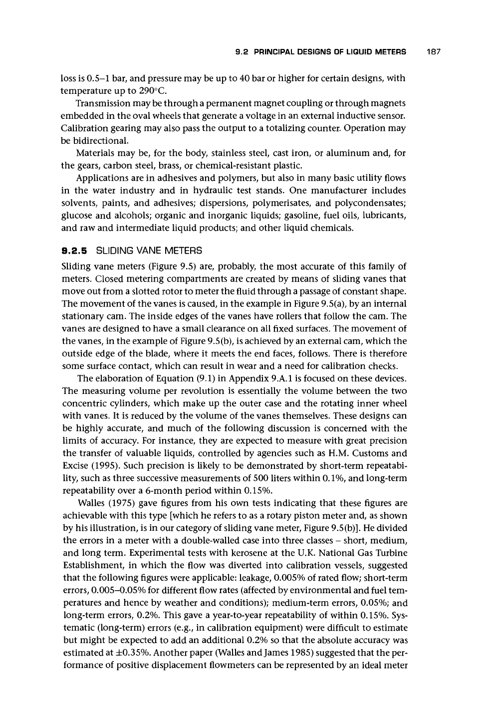
9.2.5 SLIDING VANE METERS

Sliding vane meters (Figure 9.5) are, probably, the most accurate of this family of

meters. Closed metering compartments are created by means of sliding vanes that

move out from a slotted rotor to meter the fluid through a passage of constant shape.

The movement of the vanes is caused, in the example in Figure 9.5(a), by an internal

stationary cam. The inside edges of the vanes have rollers that follow the cam. The

vanes are designed to have a small clearance on all fixed surfaces. The movement of

the vanes, in the example of Figure 9.5(b), is achieved by an external cam, which the

outside edge of the blade, where it meets the end faces, follows. There is therefore

some surface contact, which can result in wear and a need for calibration checks.

The elaboration of Equation (9.1) in Appendix 9.A.I is focused on these devices.

The measuring volume per revolution is essentially the volume between the two

concentric cylinders, which make up the outer case and the rotating inner wheel

with vanes. It is reduced by the volume of the vanes themselves. These designs can

be highly accurate, and much of the following discussion is concerned with the

limits of accuracy. For instance, they are expected to measure with great precision

the transfer of valuable liquids, controlled by agencies such as H.M. Customs and

Excise (1995). Such precision is likely to be demonstrated by short-term repeatabi-

lity, such as three successive measurements of 500 liters within

0.1%,

and long-term

repeatability over a 6-month period within 0.15%.

Walles (1975) gave figures from his own tests indicating that these figures are

achievable with this type [which he refers to as a rotary piston meter and, as shown

by his illustration, is in our category of sliding vane meter, Figure 9.5(b)]. He divided

the errors in a meter with a double-walled case into three classes - short, medium,

and long term. Experimental tests with kerosene at the U.K. National Gas Turbine

Establishment, in which the flow was diverted into calibration vessels, suggested

that the following figures were applicable: leakage, 0.005% of rated flow; short-term

errors,

0.005-0.05% for different flow rates (affected by environmental and fuel tem-

peratures and hence by weather and conditions); medium-term errors, 0.05%; and

long-term errors, 0.2%. This gave a year-to-year repeatability of within 0.15%. Sys-

tematic (long-term) errors (e.g., in calibration equipment) were difficult to estimate

but might be expected to add an additional 0.2% so that the absolute accuracy was

estimated at ±0.35%. Another paper (Walles and James 1985) suggested that the per-

formance of positive displacement flowmeters can be represented by an ideal meter

188

POSITIVE DISPLACEMENT FLOWMETERS

Cam

Measuring

Chamber

Meter

Housing

Blade

Bearing

Rotor

vanes (or blades)

measuring

chamber

(c)

Figure 9.5. Sliding vane meter: (a) Smith type showing blade (vane) path (reproduced from

Baker 1983; with permission of the author); (b) Avery Hardoll type (after the manufacturer's

literature); (c)

VAF

J5000 (reproduced with permission of

VAF

Instruments and Industrial Flow

Control Ltd.).

of arbitrary but constant volume in parallel with a small leakage that is independent

of flow rate.

Manufacturers claim very high performance in line with these published figures

0.1-0.3%.

repeatability of 0.01-0.05% for flow ranges from about 3 m

/h up to

2,000 m

/h with turndown ratio of 20:1 and size range of 64-152 mm (2.5-6 in.)

is typical. One penalty of this type of meter is its bulk and weight (60-136 kg). In

9.2 PRINCIPAL DESIGNS OF LIQUID METERS 189

some designs, the highest flow rates are achieved by ganging the meters together

in a double or triple capsule. Pressure loss should be kept to within 70-100 kPa

(10-15 psi) by suitable choice of meter size.

Materials may be cast iron for the bodies, and the rotors may be made of similar

materials or other materials such as aluminum. The same is true for outer

covers.

Low

friction ball bearings may be used. Static seals may be high nitrile, whereas dynamic

seals may also be fluorocarbon. Working pressure is about 10 bar, and temperature

ranges from about -25 to 100°C. Temperature changes cause less than 0.0015%/°C,

which is small compared with the theoretical values due to selection of materials.

The measuring chamber is fitted with pressure-balanced end covers to ensure that

there is no pressure difference across the end covers of the measuring chamber and

so to avoid distortion. Figure 9.5(c) shows a device that may also be available for 10-

to 200-mm pipe bore sizes.

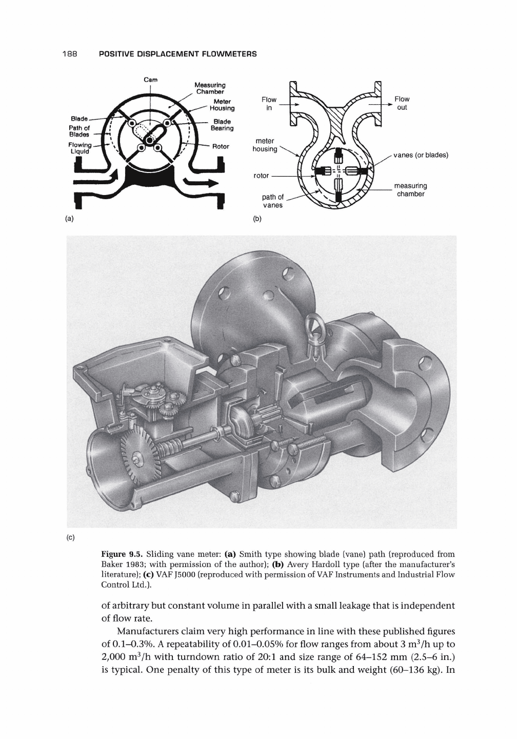
9.2.6 HELICAL ROTOR METER

Two radially pitched helical rotors trap liquid as it flows through the flowmeter caus-

ing the rotors to rotate in the longitudinal plane (Figure 9.6). Flow through the meter

is proportional to the rotational speed of the rotors. It can be used on high viscosity

liquids, but increased slippage may occur with low viscosity flows and reduce the

accuracy. The rotors form a seal with each other and with the body of the flowmeter

so that these parts must be manufactured to a high degree of precision. One man-

ufacturer (Gerrard 1979) claimed that its positive displacement meter with helical

elements had an accuracy of ±0.5% over a 150:1 flow range and a repeatability of

±0.1%.

Performance of

0.1%

rate uncertainty and

0.01%

repeatability with low effect

from viscosity are now claimed. Some designs may withstand pressures up to 230 bar,

compensate for temperature changes, and allow the passage of small solids. The use

of Equation (9.1) will require a knowledge of how many closed compartments there

are created by the two helical rotors and how many of them pass in one rotation.

One manufacturer confirms the precision level, suggesting that a higher pressure

rating is possible, with maximum flow of about 13 m

/h, an operating temperature

up to about 290°C, and viscosity up to 10

cP.

Applications are to polymers and adhesives, fuel oils, lubricating oil, blending,

hydraulic test stands, high viscosity, and thixotropic fluids. This type of meter has

also been developed for multiphase flows in North Sea oil applications (Gold et al.

1991).

Flow

Figure 9.6. Helical rotor meter (reproduced from Baker and Morris 1985; with

permission of the Institute of Measurement and Control).

190

POSITIVE DISPLACEMENT FLOWMETERS

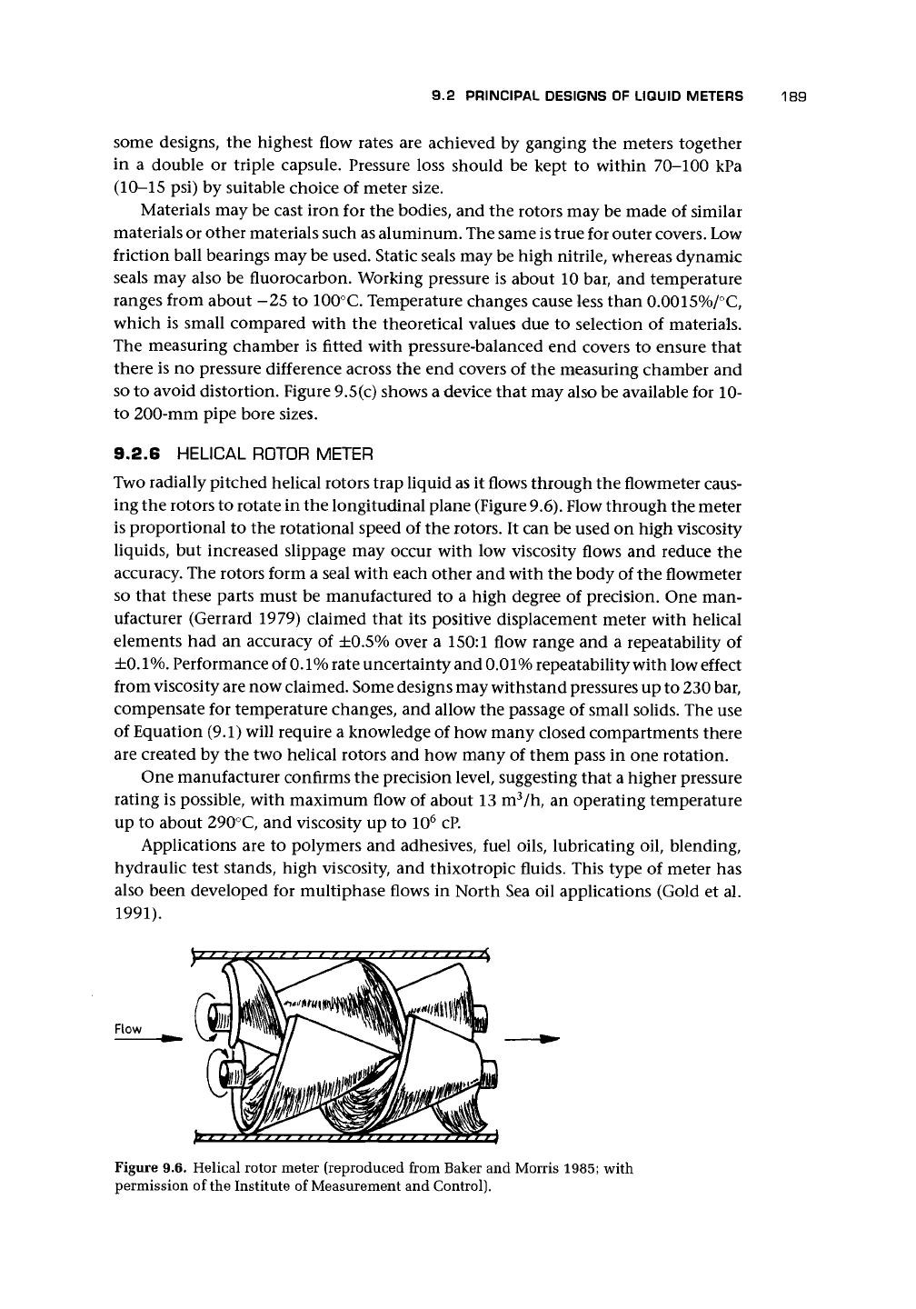
Figure 9.7. Reciprocating piston meter (reproduced from Baker and Morris

1985;

with permission of the Institute of Measurement and Control).

9.2.7

RECIPROCATING PISTON METERS

One design in which four pistons trap liquid as it passes through the flowmeter is

shown in Figure 9.7. The crankshaft rotates with a rotational speed proportional to

the flow through the meter. The liquid that passes through each cylinder in one

rotation of the shaft is equal to the swept volume of the cylinder.

Meters of this type have high accuracy claims and may also have a high pressure

drop.

The Aeroplane and Armament Experimental Establishment (Anon. 1966b)

developed a three-cylinder meter for low flows. Accuracies of ±0.5% were quoted

for kerosene flows of 9-182 1/h (2-40 gal/h) with ±2% for gasoline at rates below

32 1/h (7 gal/h). Increased slippage made high accuracy difficult to achieve at low

flows,

particularly for less viscous liquids.

One commercial producer quotes up to 33 m

/h (120 gal/min) with ±0.5% of

reading and with an

1,800:1

turndown and another down to 11/h. Viscosity may be

possible up to 30,000 cP or greater and temperatures up to about 280°C. Magnetic

couplings may be used to reduce drag and avoid a rotating seal.

Endress et al. (1989) mentioned accuracy of ±0.5 to 1% of rate, turndown of

10:1,

maximum differential pressure of 5 bar, diameter range of 25-100 mm, and

maximum pressure of 40 bar. Others may offer pressure ratings up to 200 bar.

Materials of construction may be predominantly stainless steel with seals of

Viton, Teflon, neoprene, Nordel, Buna-N, etc. Filtration to 10 /xm may be required,

and magnetic coupling may be appropriate.

Applications include gasoline pumps, pilot plants, chemical additives, engine

and hydraulic test stands, fuel consumption analysis, blending and ratio control,

and mercaptan odorant injection.

9.2.8

PRECISION GEAR FLOWMETERS

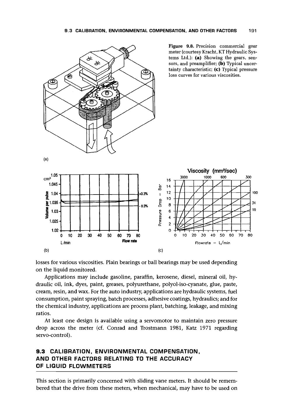
Figure 9.8(a) shows an example of

commercial device. The spaces between the gears

and the chamber wall form the fluid transfer compartments. In this version, rotation

is sensed by two electromagnetic sensors operating through a pressure-resistant and

nonmagnetic element in the housing. Two sensors can be arranged to allow bet-

ter resolution than one and to determine flow direction. Measurement uncertainty

[Figure 9.8(b)] of

±0.1%

rate is claimed. It is also claimed that rapid flow reversal can

be followed (e.g., 801/min in about 0.01 s). Meters for flow ranges of as low as 0.001

1/min and as high as 1,000 1/min may be available with temperature ranges of -30

to 150°C and pressure up to 300 bar or more. Figure 9.8(c) shows typical pressure

9.3 CALIBRATION, ENVIRONMENTAL COMPENSATION, AND OTHER FACTORS 191

1.05-

1.045-

| 1.04

£1.035

| 1.03

1.025

1.02

+0.3%

0.3%

0 10 20 30

L/min

40 50

60 70 80

Flow

rate

(b)

Figure 9.8. Precision commercial gear

meter (courtesy Kracht,

Hydraulic Sys-

tems Ltd.): (a) Showing the gears, sen-

sors,

and preamplifier; (b) Typical uncer-

tainty characteristic; (c) Typical pressure

loss curves for various viscosities.

Viscosity (mmVsec)

3000 1000 600

300

16 -

14 -

12 -

10 -

8 -

K -

0 -

1 y

^—

100

10 20 30 40 50 60 70 80

Rowrate —

L/min

(c)

losses for various viscosities. Plain bearings or ball bearings may be used depending

on the liquid monitored.

Applications may include gasoline, paraffin, kerosene, diesel, mineral oil, hy-

draulic oil, ink, dyes, paint, greases, polyurethane, polyol-iso-cyanate, glue, paste,

cream, resin, and wax. For the auto industry, applications are hydraulic systems, fuel

consumption, paint spraying, batch processes, adhesive coatings, hydraulics; and for

the chemical industry, applications are process plant, batching, leakage, and mixing

ratios.

At least one design is available using a servomotor to maintain zero pressure

drop across the meter (cf. Conrad and Trostmann 1981, Katz 1971 regarding

servo-control).

9.3 CALIBRATION, ENVIRONMENTAL COMPENSATION,

AND OTHER FACTORS RELATING TO THE ACCURACY

OF LIQUID FLOWMETERS

This section is primarily concerned with sliding vane meters. It should be remem-

bered that the drive from these meters, when mechanical, may have to be used on

192 POSITIVE DISPLACEMENT FLOWMETERS

Leakage

Bypass

0.8

0.6

0.4

0.2

Mechanical

friction

20 40 60 80

URV

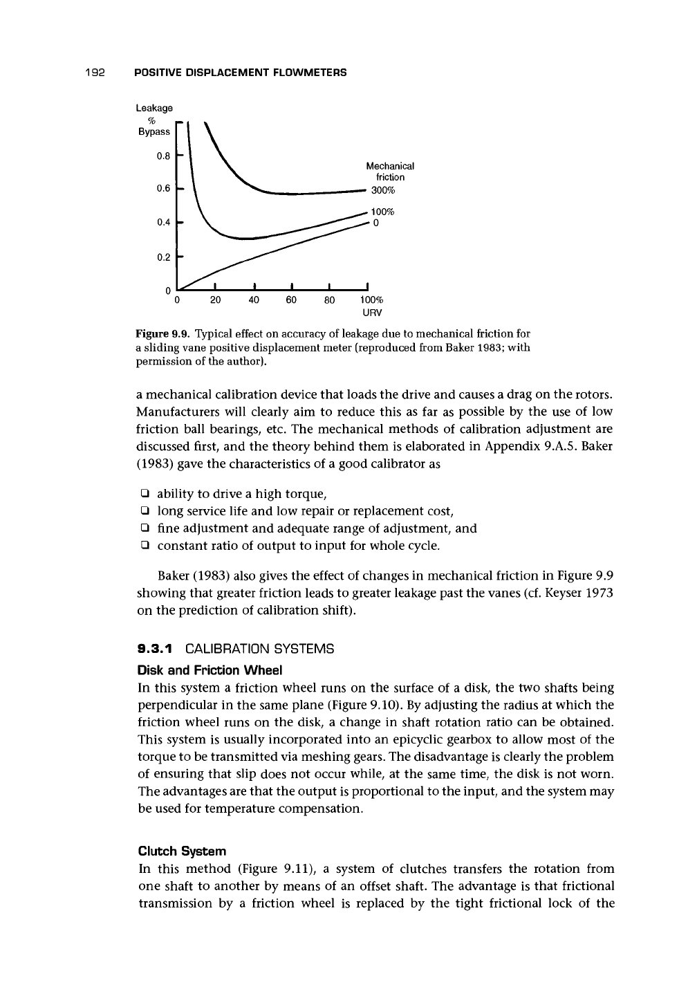
Figure 9.9. Typical effect on accuracy of leakage due to mechanical friction for

a sliding vane positive displacement meter (reproduced from Baker 1983; with

permission of the author).

a mechanical calibration device that loads the drive and causes a drag on the rotors.

Manufacturers will clearly aim to reduce this as far as possible by the use of low

friction ball bearings, etc. The mechanical methods of calibration adjustment are

discussed first, and the theory behind them is elaborated in Appendix 9.A.5. Baker

(1983) gave the characteristics of a good calibrator as

• ability to drive a high torque,

• long service life and low repair or replacement cost,

• fine adjustment and adequate range of adjustment, and

• constant ratio of output to input for whole cycle.

Baker (1983) also gives the effect of changes in mechanical friction in Figure 9.9

showing that greater friction leads to greater leakage past the vanes (cf. Keyser 1973

on the prediction of calibration shift).

9.3.1 CALIBRATION SYSTEMS

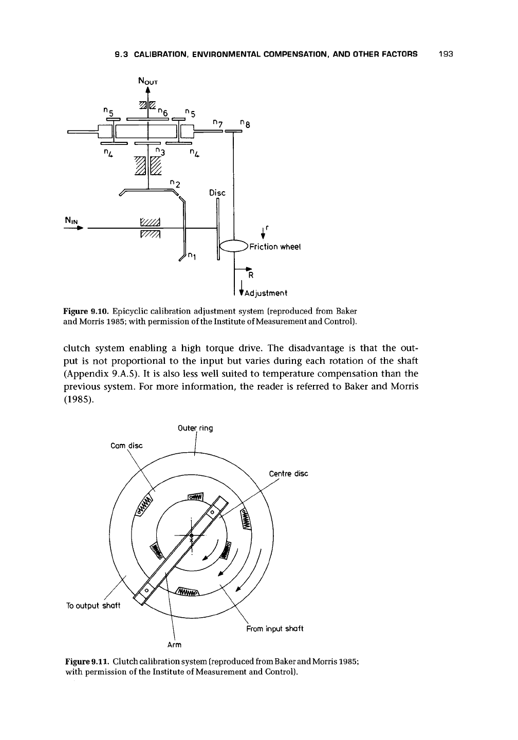
Disk and Friction Wheel

In this system a friction wheel runs on the surface of a disk, the two shafts being

perpendicular in the same plane (Figure 9.10). By adjusting the radius at which the

friction wheel runs on the disk, a change in shaft rotation ratio can be obtained.

This system is usually incorporated into an epicyclic gearbox to allow most of the

torque to be transmitted via meshing gears. The disadvantage is clearly the problem

of ensuring that slip does not occur while, at the same time, the disk is not worn.

The advantages are that the output is proportional to the input, and the system may

be used for temperature compensation.

Clutch System

In this method (Figure 9.11), a system of clutches transfers the rotation from

one shaft to another by means of an offset shaft. The advantage is that frictional

transmission by a friction wheel is replaced by the tight frictional lock of the

9.3 CALIBRATION, ENVIRONMENTAL COMPENSATION, AND OTHER FACTORS 193

Adjustment

Figure 9.10. Epicyclic calibration adjustment system (reproduced from Baker

and Morris

1985;

with permission of the Institute of Measurement and Control).

clutch system enabling a high torque drive. The disadvantage is that the out-

put is not proportional to the input but varies during each rotation of the shaft

(Appendix 9.A.5). It is also less well suited to temperature compensation than the

previous system. For more information, the reader is referred to Baker and Morris

(1985).

Outer ring

Cam disc

output shaft

Centre disc

From input shaft

Arm

Figure

9.11.

Clutch calibration system (reproduced from Baker and Morris 1985;

with permission of the Institute of Measurement and Control).

194

POSITIVE DISPLACEMENT FLOWMETERS

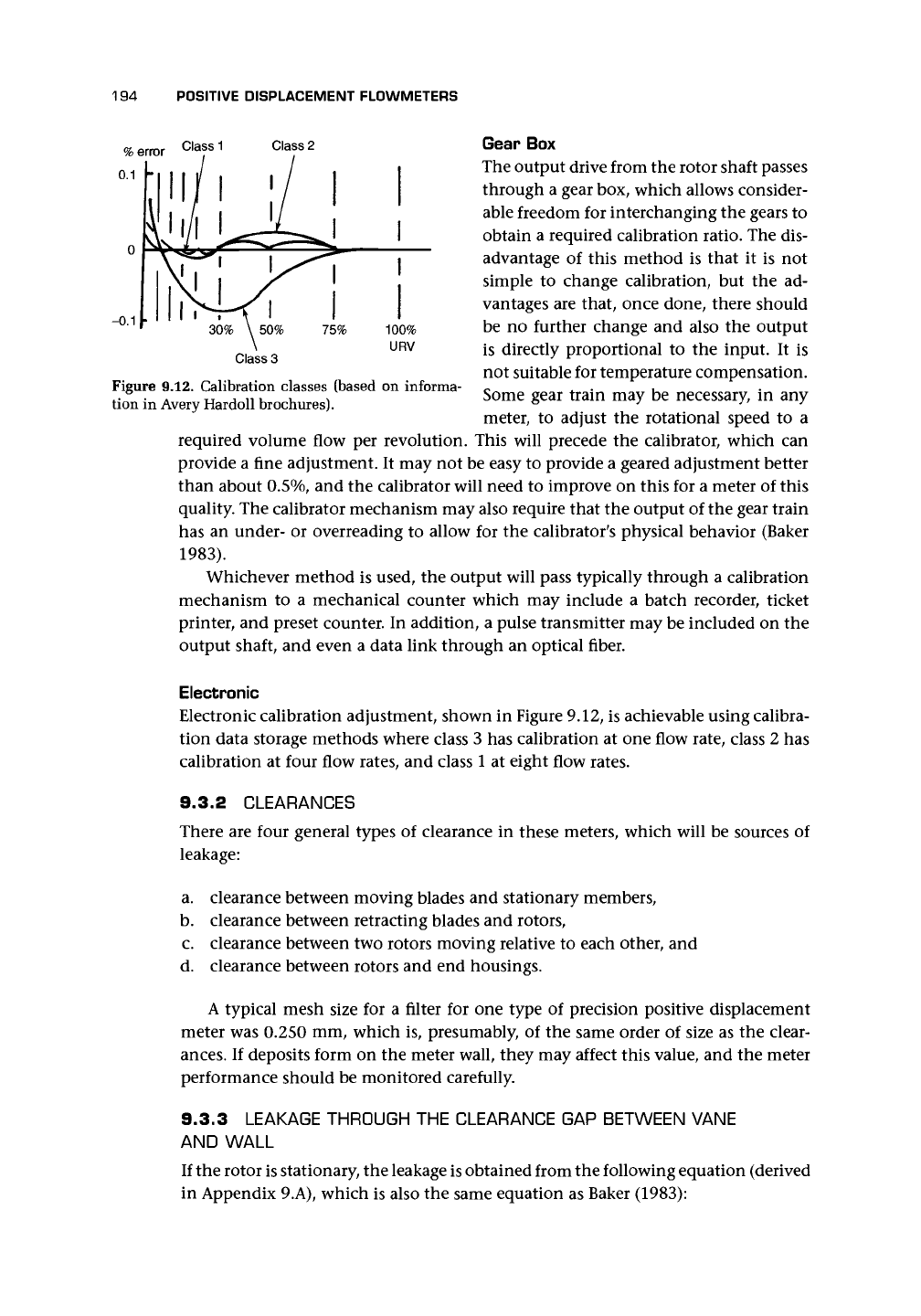
Class 1

Class 2

-0.1

75%

Class 3

100%

URV

Figure 9.12. Calibration classes (based on informa-

tion in Avery Hardoll brochures).

Gear Box

The output drive from the rotor shaft passes

through a gear box, which allows consider-

able freedom for interchanging the gears to

obtain a required calibration ratio. The dis-

advantage of this method is that it is not

simple to change calibration, but the ad-

vantages are that, once done, there should

be no further change and also the output

is directly proportional to the input. It is

not suitable for temperature compensation.

Some gear train may be necessary, in any

meter, to adjust the rotational speed to a

required volume flow per revolution. This will precede the calibrator, which can

provide a fine adjustment. It may not be easy to provide a geared adjustment better

than about 0.5%, and the calibrator will need to improve on this for a meter of this

quality. The calibrator mechanism may also require that the output of the gear train

has an under- or overreading to allow for the calibrator's physical behavior (Baker

1983).

Whichever method is used, the output will pass typically through a calibration

mechanism to a mechanical counter which may include a batch recorder, ticket

printer, and preset counter. In addition, a pulse transmitter may be included on the

output shaft, and even a data link through an optical fiber.

Electronic

Electronic calibration adjustment, shown in Figure 9.12, is achievable using calibra-

tion data storage methods where class 3 has calibration at one flow rate, class 2 has

calibration at four flow rates, and class 1 at eight flow rates.

9.3.2 CLEARANCES

There are four general types of clearance in these meters, which will be sources of

leakage:

a. clearance between moving blades and stationary members,

clearance between retracting blades and rotors,

c. clearance between two rotors moving relative to each other, and

d. clearance between rotors and end housings.

A typical mesh size for a filter for one type of precision positive displacement

meter was 0.250 mm, which is, presumably, of the same order of size as the clear-

ances.

If deposits form on the meter wall, they may affect this value, and the meter

performance should be monitored carefully.

9.3.3 LEAKAGE THROUGH THE CLEARANCE GAP BETWEEN VANE

AND WALL

If the rotor is stationary, the leakage is obtained from the following equation (derived

in Appendix 9.A), which is also the same equation as Baker (1983):

9.3 CALIBRATION, ENVIRONMENTAL COMPENSATION, AND OTHER FACTORS

195

^slip = 7^ z ~ {y.Z)

IZ/JL

Ideally, the liquid in the gap would be car-

ried at the same speed as the rotor blade,

and so the leakage when the vanes are mov-

ing is

^leakage

— \ "^

(9.3)

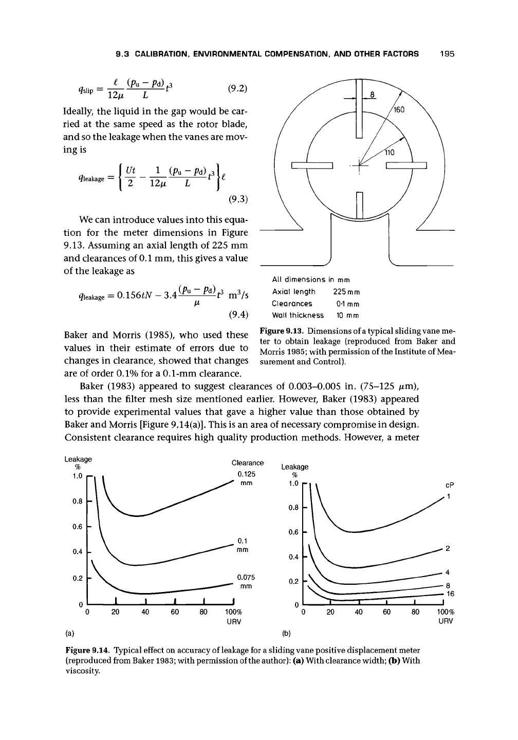
We can introduce values into this equa-

tion for the meter dimensions in Figure

9.13.

Assuming an axial length of 225 mm

and clearances of

0.1

mm, this gives a value

of the leakage as

^leakage

= ^

(9.4)

All

dimensions

in mm

Axial

length

225mm

Clearances

0-1 mm

Wall

thickness

10 mm

Figure 9.13. Dimensions of

typical sliding vane me-

ter to obtain leakage (reproduced from Baker and

Morris

1985;

with permission of the Institute of Mea-

surement and Control).

Baker and Morris (1985), who used these

values in their estimate of errors due to

changes in clearance, showed that changes

are of order

0.1%

for a 0.1-mm clearance.

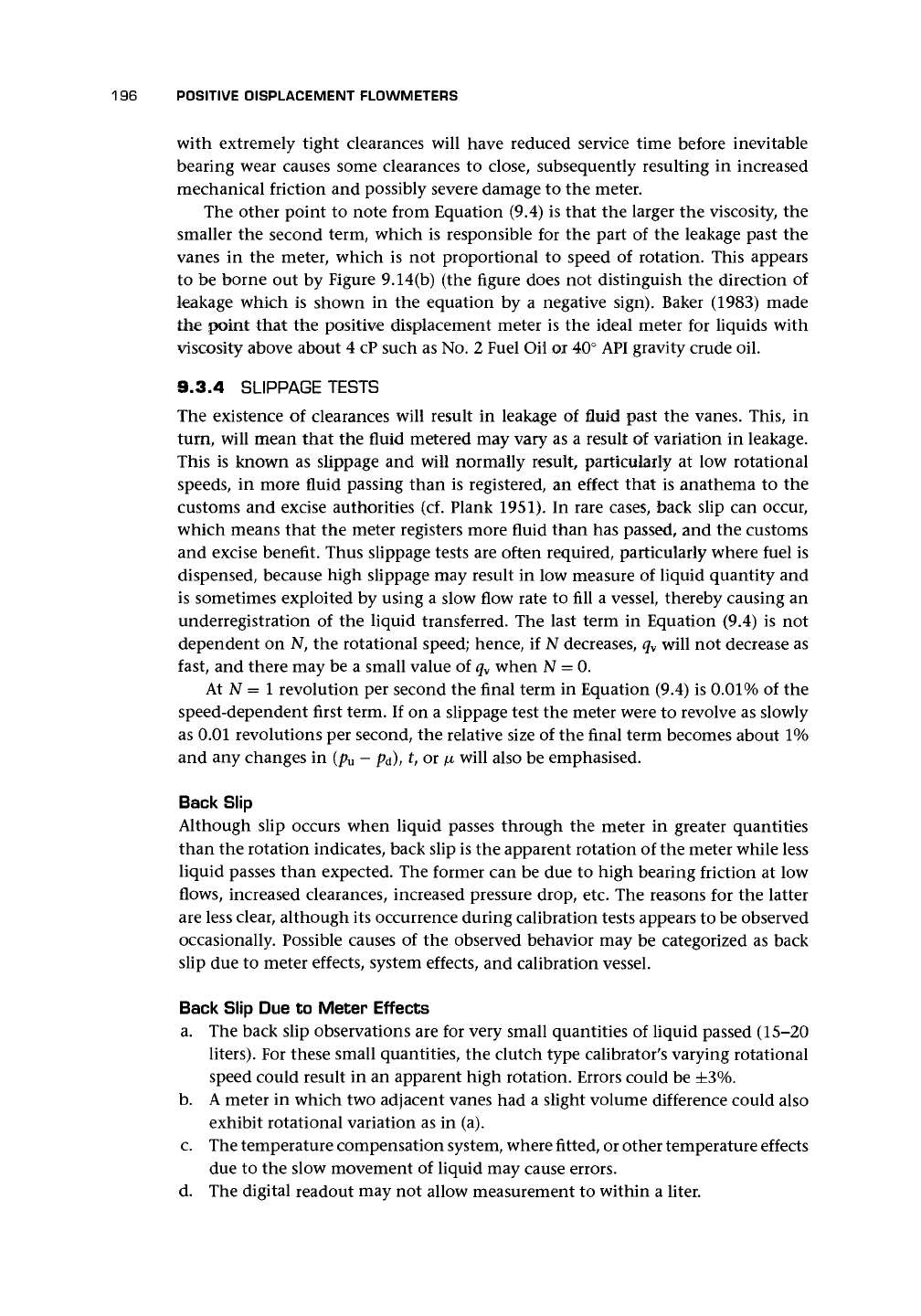
Baker (1983) appeared to suggest clearances of 0.003-0.005 in. (75-125 /xm),

less than the filter mesh size mentioned earlier. However, Baker (1983) appeared

to provide experimental values that gave a higher value than those obtained by

Baker and Morris [Figure 9.14(a)]. This is an area of necessary compromise in design.

Consistent clearance requires high quality production methods. However, a meter

Clearance

0.125

20 40 60

80 100%

URV

(b)

Figure 9.14. Typical effect on accuracy of leakage for a sliding vane positive displacement meter

(reproduced from Baker

1983;

with permission of the

author):

(a) With clearance width; (b) With

viscosity.

19B POSITIVE DISPLACEMENT FLOWMETERS

with extremely tight clearances will have reduced service time before inevitable

bearing wear causes some clearances to close, subsequently resulting in increased

mechanical friction and possibly severe damage to the meter.

The other point to note from Equation (9.4) is that the larger the viscosity, the

smaller the second term, which is responsible for the part of the leakage past the

vanes in the meter, which is not proportional to speed of rotation. This appears

to be borne out by Figure 9.14(b) (the figure does not distinguish the direction of

leakage which is shown in the equation by a negative sign). Baker (1983) made

the point that the positive displacement meter is the ideal meter for liquids with

viscosity above about 4 cP such as No. 2 Fuel Oil or 40° API gravity crude oil.

9.3.4 SLIPPAGE TESTS

The existence of clearances will result in leakage of fluid past the vanes. This, in

turn, will mean that the fluid metered may vary as a result of variation in leakage.

This is known as slippage and will normally result, particularly at low rotational

speeds, in more fluid passing than is registered, an effect that is anathema to the

customs and excise authorities (cf. Plank 1951). In rare cases, back slip can occur,

which means that the meter registers more fluid than has passed, and the customs

and excise benefit. Thus slippage tests are often required, particularly where fuel is

dispensed, because high slippage may result in low measure of liquid quantity and

is sometimes exploited by using a slow flow rate to fill a vessel, thereby causing an

underregistration of the liquid transferred. The last term in Equation (9.4) is not

dependent on N, the rotational speed; hence, if N decreases, q

will not decrease as

fast, and there may be a small value of q

when N = 0.

At N = 1 revolution per second the final term in Equation (9.4) is 0.01% of the

speed-dependent first term. If on a slippage test the meter were to revolve as slowly

as 0.01 revolutions per second, the relative size of the final term becomes about 1%

and any changes in (p

—

pa),

t, or /x will also be emphasised.

Back Slip

Although slip occurs when liquid passes through the meter in greater quantities

than the rotation indicates, back slip is the apparent rotation of the meter while less

liquid passes than expected. The former can be due to high bearing friction at low

flows, increased clearances, increased pressure drop, etc. The reasons for the latter

are less clear, although its occurrence during calibration tests appears to be observed

occasionally. Possible causes of the observed behavior may be categorized as back

slip due to meter effects, system effects, and calibration vessel.

Back Slip Due to Meter Effects

a. The back slip observations are for very small quantities of liquid passed (15-20

liters).

For these small quantities, the clutch type calibrator's varying rotational

speed could result in an apparent high rotation. Errors could be ±3%.

A meter in which two adjacent vanes had a slight volume difference could also

exhibit rotational variation as in (a).

c. The temperature compensation system, where fitted, or other temperature effects

due to the slow movement of liquid may cause errors.

d. The digital readout may not allow measurement to within a liter.