Bernatz R. Fourier Series and Numerical Methods for Partial Differential Equations

Подождите немного. Документ загружается.

92 STURM-LIOUVILLE PROBLEMS

so this sequence does not eventually become zero from some index j forward. If

—

1, then

0(0 + 1)-1(1 + 1) 1

C2 = C0+2 =

(0 + 1X0 + 2) °°

and

2(2 + 1)-1(1 + 1) 5

C4 = C2+2 =

(2 + l)(2 + 2)

C0 =

so none of the coefficients c

j, j = 1,2,3,... are zero. However,

1(1 + 1)-1(1 + 1) 0

C3 = Cl+2 =

(1 + 1K1 + 2)

Cl =

C1 =

so each coefficient c

j+i,j

—

2,3,...

is zero.

The results demonstrated in the previous paragraph can be generalized to say that

if λ = ra(ra + 1) for any positive, odd integer ra, then

i) The function θι(χ) becomes the mth-order Legendre polynomial

(x) = θι(χ) = cix + c

+ · · · + c

(3.52)

with the total number of terms in the polynomial equal to .

ii) The function ©2(0;) is nonterminating and is referred to as the Legendre

function of the second kind denoted as Q

(x).

If m is any positive, even integer, then

i) The function θι(χ) is nonterminating and is referred to as the Legendre func-

tion of the second kind denoted as Q

(x),

ii) The function θ2(χ) becomes the mth-order Legendre polynomial

(x) = θ

(χ) = c

x + c

+ · · · + c

(3.53)

m + 2

with the total number of terms in the polynomial equal to .

A single expression for the Legendre polynomials given in Equations (3.52) and

(3.53) can be derived with the additional property that each polynomial takes the value

of unity at x=\. Without providing the details of

the

development, the expression for

the nth Legendre polynomial P

(x) is

n(*0 = ¿E^-,

{2n

■„*"-*

(n = 0,l,2,...) (3.54)

where the upper index m is determined by

{

—

l)/2 if n is odd

n/2 if n is even

EXERCISES 93

' i !

/ i

-OÄ-0.4

-0.2,"

v 02 0.4 yO.6 Λ.8 1

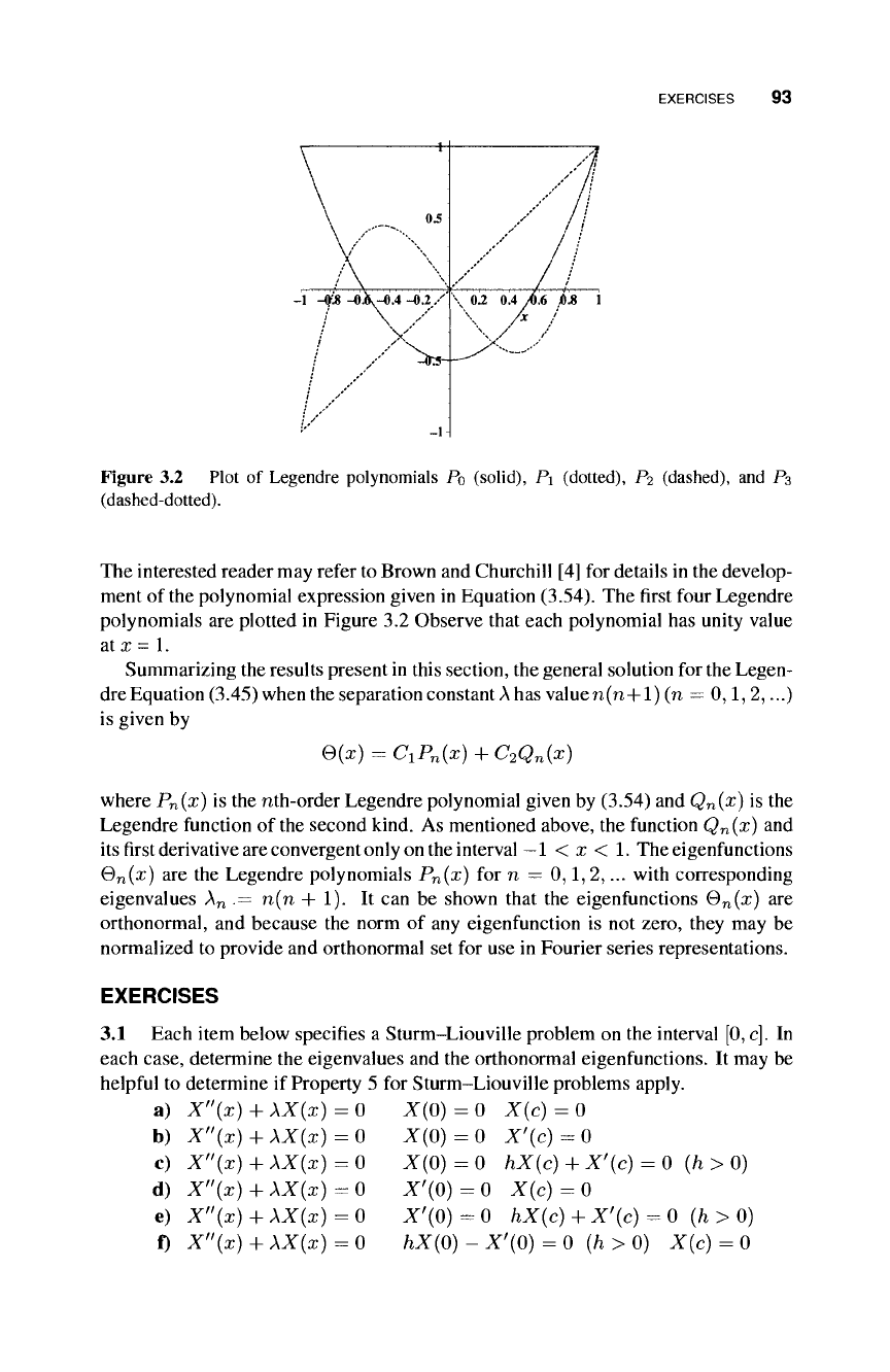
Figure 3.2 Plot of Legendre polynomials Po (solid), P\ (dotted),

P<¿

(dashed), and P3

(dashed-dotted).

The interested reader may refer to Brown and Churchill [4] for details in the develop-

ment of the polynomial expression given in Equation (3.54). The first four Legendre

polynomials are plotted in Figure 3.2 Observe that each polynomial has unity value

at x

Summarizing the results present in this section, the general solution for the Legen-

dre Equation (3.45) when the separation constant λ has value n(n-f

(n =

0,1,2,...)

is given by

e(x)

(x)

Qn(x)

where P

{x) is the nth-order Legendre polynomial given by (3.54) and Q

(x) is the

Legendre function of the second kind. As mentioned above, the function Q

(x) and

its

first

derivative are convergent only on the interval

— 1

< x < 1. The eigenfunctions

(χ) are the Legendre polynomials P

{x) for n — 0,1,2,... with corresponding

eigenvalues λ

.= n(n + 1). It can be shown that the eigenfunctions θ

(χ) are

orthonormal, and because the norm of any eigenfunction is not zero, they may be

normalized to provide and orthonormal set for use in Fourier series representations.

EXERCISES

3.1 Each item below specifies a Sturm-Liouville problem on the interval

[0, c].

each case, determine the eigenvalues and the orthonormal eigenfunctions. It may be

helpful to determine if Property 5 for Sturm-Liouville problems apply.

a) Χ"(χ) + ΧΧ(χ)=0 Χ(0)=0 X(c)=0

X(0) = 0

X'(Q)

= 0

X'(0)

= 0

b) Χ"(χ) + λΧ(χ) = 0

c) X"{x) + XX(x) = 0

d) X"(x) + XX(x) = 0

e) Χ"(χ) + λΧ(χ)==0

f) X"(x) + XX(x)=0

X'(c)

- 0

hX(c)+X'(c) = 0 (ft>0)

X(c) = 0

hX(c)

X'(c) - 0 (ft > 0)

hX{0) - X'(0) =0 (ft > 0) X{c) = 0

94 STURM-LIOUVILLE PROBLEMS

3.2 The differential equation

y" + Bxy' + Cy = 0

where τ4, 5, and C are constants, is called the Cauchy-Euler equation. Make

the substitution x = e

to show that this equation may be transformed into the

constant-coefficient differential equation

d2y

+(R A\

¿H

(*-^

»=°

3.3 Consider the Regular Sturm-Liouville problem given below.

[xX'(x)Y + -X(x) = 0 (1< x < b)

X(l) = 0, X(b) = 0

a) Write the differential equation in Cauchy-Euler form (see Exercise 3.2).

b) Transform the Cauchy-Euler equation found in the previous step to the form

—2-+λΧ = 0 (0<s<lnb)

with transformed boundary conditions

= 0) = 0 X(s = \nb) =0

using the substitution x

—

c) Use the result from an appropriate Sturm-Liouville problem to determine

the eigenvalues and eigenfunctions of the original Sturm-Liouville problem

of this exercise are

= k

(x) =

sin(k

lnx) (n = 1, 2,

3,...)

where k

= ηπ / In b.

d) Verify the eigenfunctions found in the previous part are orthogonal on the

interval 1 < x < b with respect to the weight function p(x) = 1/x. (Hint:

make the substitution s — (π/ In

In x once you have set up the integral.

The result of Exercise 2.24 is useful as well.)

3.4 The following Sturm-Liouville problems are singular because of the semi-

infinite or infinite interval for x. Such intervals result in applications where tempera-

ture,

for

example,

is dependent on a spatial variable that is not bounded in one or either

direction. Solve the given problem to determine all eigenvalues and eigenfunctions.

In all cases, M is a fixed positive real number and assume λ is real.

X'\x)

+ XX(x) = 0 x > 0 X(0) = 0 and

\X(x)\

< M

EXERCISES 95

X"{x)

+ XX(x) = 0 x > 0 X'(0) = 0 and |X(x)| < M

X"(x) + AX(x) = 0 -oo<x<oo \X(x)\<M

3.5 Provide the details to show how the change of variable x = cos

results in

Equation (3.45) from Equation (3.44).

3.6 Use Equation (3.47) and the ratio test for series convergence to show the series

given in Equation (3.50) converges for x

< 1.

This Page Intentionally Left Blank

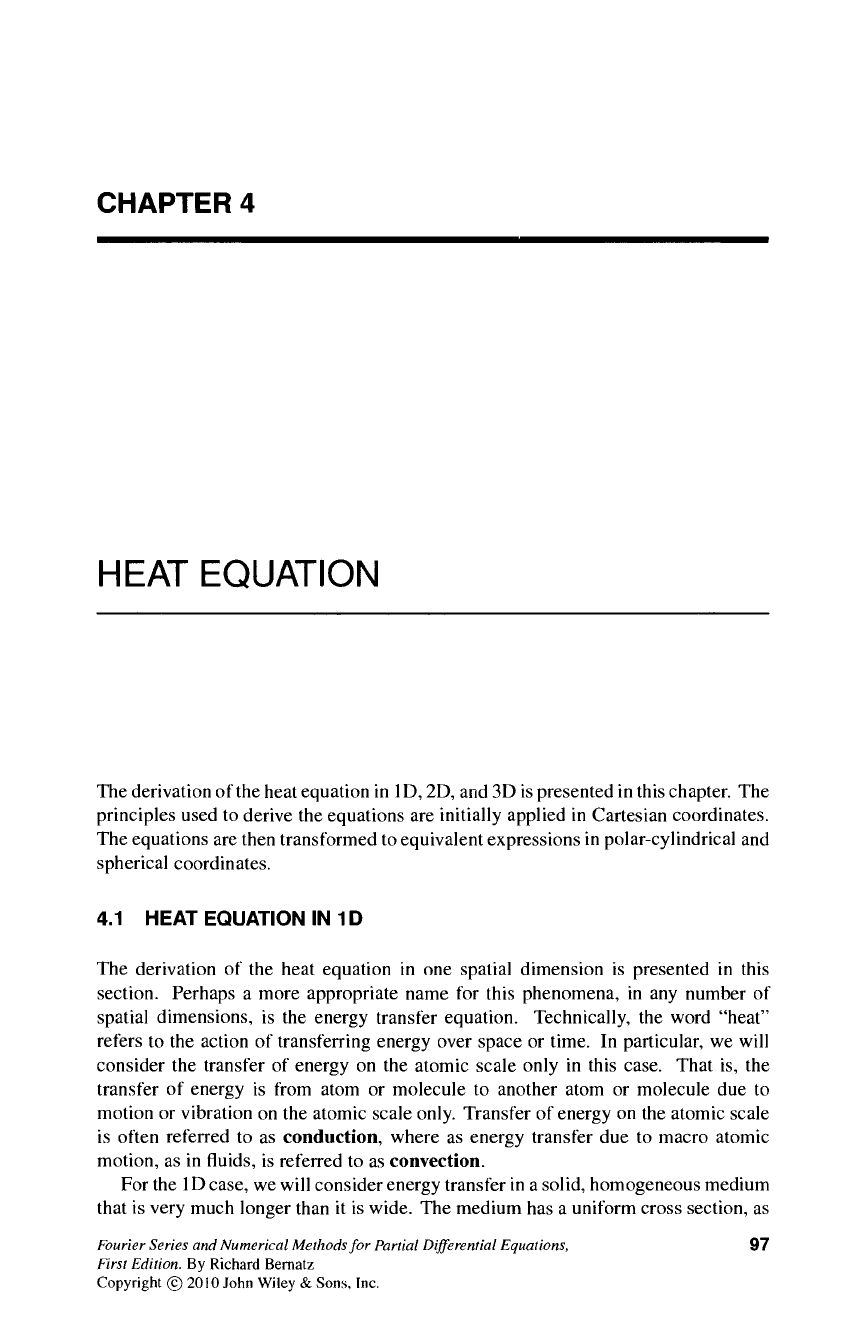
CHAPTER 4

HEAT EQUATION

The derivation of

the

heat equation in ID, 2D, and 3D is presented in this chapter. The

principles used to derive the equations are initially applied in Cartesian coordinates.

The equations are then transformed to equivalent expressions in polar-cylindrical and

spherical coordinates.

4.1 HEAT EQUATION IN 1D

The derivation of the heat equation in one spatial dimension is presented in this

section. Perhaps a more appropriate name for this phenomena, in any number of

spatial dimensions, is the energy transfer equation. Technically, the word "heat"

refers to the action of transferring energy over space or time. In particular, we will

consider the transfer of energy on the atomic scale only in this case. That is, the

transfer of energy is from atom or molecule to another atom or molecule due to

motion or vibration on the atomic scale only. Transfer of energy on the atomic scale

is often referred to as conduction, where as energy transfer due to macro atomic

motion, as in fluids, is referred to as convection.

For the

case, we will consider energy transfer in a solid, homogeneous medium

that is very much longer than it is wide. The medium has a uniform cross section, as

Fourier Series and Numerical Methods for Partial Differential Equations, 97

First Edition. By Richard Bernatz

98 HEAT EQUATION

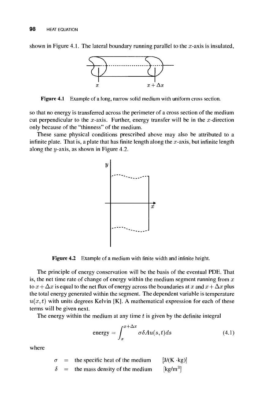
shown in Figure

4.1.

The lateral boundary running parallel to the x-axis is insulated,

x x + Ax

Figure

4.1

Example of

long, narrow solid medium with uniform cross section.

so that no energy is transferred across the perimeter of a cross section of the medium

cut perpendicular to the x-axis. Further, energy transfer will be in the x-direction

only because of the "thinness" of the medium.

These same physical conditions prescribed above may also be attributed to a

infinite plate. That is, a plate that has finite length along the x-axis, but infinite length

along the y-axis, as shown in Figure 4.2.

* "*** **-"

**"*---.--·

Figure 4.2 Example of

medium with

finite

width and infinite height.

The principle of energy conservation will be the basis of the eventual PDE. That

is,

the net time rate of change of energy within the medium segment running from x

to x

Δχ is equal to the net flux of energy across the boundaries at x and x + Δχ plus

the total energy generated within the segment. The dependent variable is temperature

u(x,t) with units degrees Kelvin [K]. A mathematical expression for each of these

terms will be given next.

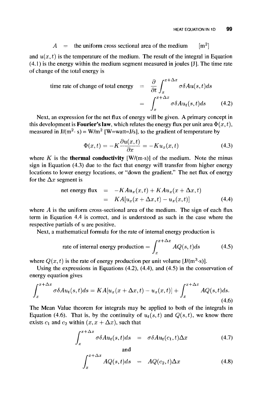
The energy within the medium at any time t is given by the definite integral

/»χ+Δχ

energy = / a5Au(s,t)ds (4.1)

J x

where

σ — the specific heat of the medium [J/(K kg)]

δ = the mass density of the medium [kg/m

]

HEAT

EQUATION

IN 1D 99

A = the uniform cross sectional area of the medium [m

]

and u(x, t) is the temperature of the medium. The result of the integral in Equation

(4.1) is the energy within the medium segment measured in joules [J]. The time rate

of change of the total energy is

ß px+Ax

time rate of change of total energy = — / a5Au(s, t)ds

v* J x

x-\-Ax

a6Au

(s,t)ds (4.2)

Next, an expression for the net flux of energy will be given. A primary concept in

this development is Fourier's law, which relates the energy flux per unit area Φ(χ, £),

measured in J/(m

· s) = W/m

[W=watt=J/s], to the gradient of temperature by

Φ(χ, ί) = -K^^- = -Ku

(x, t) (4.3)

where K is the thermal conductivity [W/(ms)] of the medium. Note the minus

locations to lower energy locations, or "down the gradient." The net flux of energy

for the Δχ segment is

net energy flux = —KAu

(x, t) + KAu

(x + Δχ, i)

= KA[u

(x -f Ax,t) - u

(x,t)} (4.4)

where A is the uniform cross-sectional area of the medium. The sign of each flux

term in Equation 4.4 is correct, and is understood as such in the case where the

respective partíais of u are positive.

Next, a mathematical formula for the rate of internal energy production is

ΛΧ+ΔΧ

rate of internal energy production = / AQ(s, t)ds (4.5)

J x

where Q(x,t) is the rate of energy production per unit volume [J/(m

s)].

Using the expressions in Equations (4.2), (4.4), and (4.5) in the conservation of

energy equation gives

px-\-Ax px+Ax

j aSAu

(s,t)ds = KA[u

(x + Δχ,ί)

—

(x,t)] + / AQ(s,t)ds.

J X J X

(4.6)

The Mean Value theorem for integrals may be applied to both of the integrals in

Equation (4.6). That is, by the continuity of u

(s,t) and Q(s,t), we know there

exists c\ and c

within (x, x + Ax), such that

fX+Ax

aSAu

(s,t)ds = aSAut(ci,t)Ax (4.7)

J x

and

x-\-Ax

AQ(s,t)ds = AQ(c

,t)Ax (4.8)

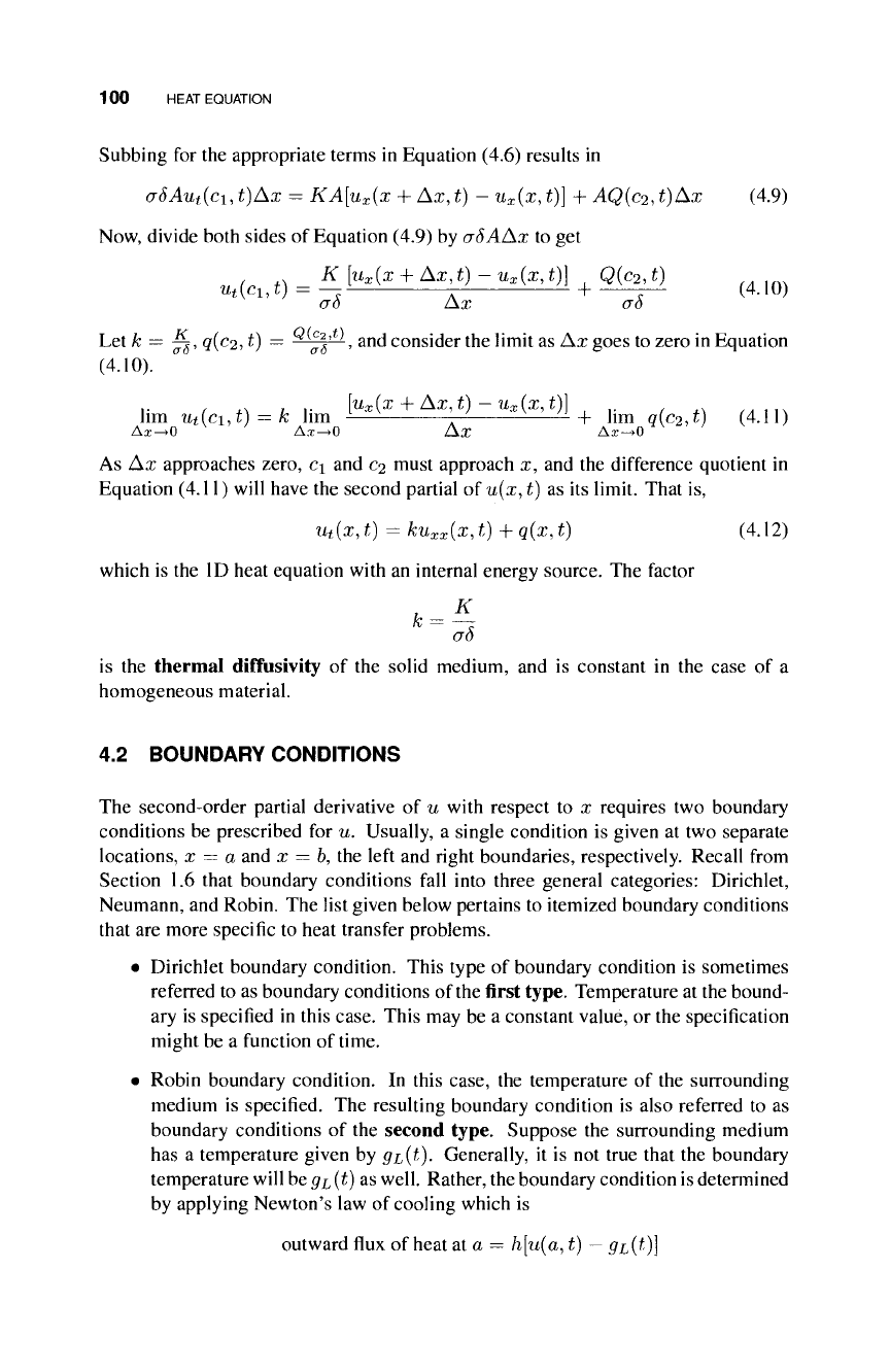
100 HEAT EQUATION

Subbing for the appropriate terms in Equation (4.6) results in

aSAut(ci,t)Ax = KA[u

(x + Δχ,t) - u

(x,t)] + AQ(c

,t)Ax (4.9)

Now, divide both sides of Equation (4.9) by σδΑΑχ to get

K[u

(x + Ax,t)-u

(x,t)\

σδ Ax σο

Let k = ^, q(c

,t) = ^

, and consider the limit as Ax goes to zero in Equation

(4.10).

lim ut(c

t) = k Urn M* +As,t) - M*,*)]

Δχ^Ο

Δ,τ^Ο Δχ Δχ-^0

As Ax approaches zero, c\ and c

must approach x, and the difference quotient in

Equation (4.11) will have the second partial of u(x, t) as its limit. That is,

(x,t) = ku

(x,t) + q(x,t) (4.12)

which is the ID heat equation with an internal energy source. The factor

is the thermal diffusivity of the solid medium, and is constant in the case of a

homogeneous material.

4.2 BOUNDARY CONDITIONS

The second-order partial derivative of u with respect to x requires two boundary

conditions be prescribed for u. Usually, a single condition is given at two separate

locations, x — a and x — b, the left and right boundaries, respectively. Recall from

Section 1.6 that boundary conditions fall into three general categories: Dirichlet,

Neumann, and Robin. The list given below pertains to itemized boundary conditions

that are more specific to heat transfer problems.

• Dirichlet boundary condition. This type of boundary condition is sometimes

referred to as boundary conditions of

the

first type. Temperature at the bound-

ary is specified in this case. This may be a constant value, or the specification

might be a function of time.

• Robin boundary condition. In this case, the temperature of the surrounding

medium is specified. The resulting boundary condition is also referred to as

boundary conditions of the second type. Suppose the surrounding medium

has a temperature given by

#L(¿)·

Generally, it is not true that the boundary

temperature will be

(t) as well. Rather, the boundary condition is determined

by applying Newton's law of cooling which is

outward flux of heat at a = h[u(a, t)

— gL,(t)]

HEAT EQUATION IN 2D 101

where h is the heat exchange coefficient. Recall that the flux of heat at the

left boundary may also be expressed in terms of w

(a, t) through Fourier's law.

That is,

outward flux of heat at a = Ku

(a, t)

where K is the thermal conductivity of the object. Note this equation indicates

the outward flux is positive if the partial of u is positive at the boundary. That

is to say, if the object is warmer that the surrounding medium (u

{a, t) > 0),

then the flux of heat is in an outward direction.

Equating these two expressions for outward flux of heat at x = a gives

(a,t) = h[u(a,t)

-#L(¿)]

(a,t) = —\u(a,t) -9L(t)]

• Neumann boundary condition. Sometimes referred to as a boundary condition

of the third type, the flux of energy normal to the boundary and into the

domain is specified in this case. Insulated boundaries are those in which no

energy is transferred. In the ID case this means u

(a)

= 0. More generally, the

boundary flux may be a function of time t so that one would have u

(a) —

f(t).

4.3 HEAT EQUATION IN 2D

The derivation of the heat transfer equation in two spatial dimensions is presented

in this section. The development is quite similar to the ID case in that the total

change of heat within a 2D Cartesian differential control volume is given equal to

the net flux of heat in the two Cartesian directions plus the internal source (or sink)

of energy. Figure 4.3 shows the differential 2D Cartesian control volume that is a

representative of an arbitrarily small control volume from within the solid medium

under consideration.

The total energy within the control volume is given by

px+Ax py+Ay

/ / a5Hu(r,s,t)dsdr

J x Jy

where

σ = the specific heat of the medium [J/(K kg)]

δ = the mass density of the medium [kg/m

]

H = the uniform thickness of the medium [m]

and u(r, s, t) is the temperature of the medium as a function of x location r, y location

and time t. Note that, as in the case of the ID derivation, the integral gives the

energy within the differential control volume in joules [J].