Devore J.L., Berk K.N. Modern Mathematical Statistics with Applications

Подождите немного. Документ загружается.

The result of this integration is

3;5

ðy

; y

Þ¼

2!1!1!

½Fðy

Þ

½Fðy

ÞFðy

Þ

½1  Fðy

Þ

f ð y

Þf ðy

1< y

< y

< 1

In the general case, the numerator in the leading expression involving factorials

becomes n! and the denominator becomes i  1ðÞ! j  i  1ðÞ! n  jðÞ!: The three

exponents on bracketed terms change in a corresponding way .

An Intuitive Derivation of Order Statistic PDF’s

Let D be a number quite close to 0, and consider the three class intervals

1; yð; y; y þ Dð, and y þ D; 1ðÞ. For a sing le X, the probabilities of these

three classes are

¼ FðyÞ p

yþD

f ð xÞdx f ðyÞD p

¼ 1  Fðy þ DÞ

For a random sample of size n, it is very unlikely that two or more X’s will fall in

the second interval. The probability that the ith order statistic falls in the second

interval is then approximately the probability that i  1 of the X’s are in the

first interval, one is in the second, and the remaining n  iX’s are in the third

class. This is just a multinomial probability:

Pðy < Y

 y þ DÞ

ði  1Þ!1!ðn  iÞ!

½Fðy

Þ

i1

 f ðyÞD½1  Fðy þ DÞ

ni

Dividing both sides by D and taking the limit as D ! 0 gives exactly the pdf of Y

obtained earli er via integration.

Similar reasoning works with the joint pdf of Y

and Y

(i < j). In this

case there are five relevant class intervals: ð1; y

; y

; y

þ D

ð; y

þ D

; y



;

; y

þ D



; and ðy

þ D

; 1Þ

Exercises Section 5.5 (65–77)

65. A friend of ours takes the bus five days per week

to her job. The five waiting times until she can

board the bus are a random sample from a uniform

distribution on the interval from 0 to 10 min.

a. Determine the pdf and then the expected

value of the largest of the five waiting times.

b. Determine the expected value of the differ-

ence between the largest and smallest times.

c. What is the expected value of the sample

median waiting time?

d. What is the standard deviation of the largest

time?

66. Refer back to example 5.29. Because n ¼ 4, the

sample median is (Y

+ Y

)/2. What is the

expected value of the sample median, and how

does it compare to the median of the population

distribution?

67. Referring back to Exercise 65, suppose you learn

that the smallest of the five waiting times is 4

min. What is the conditional density function of

the largest waiting time, and what is the expected

value of the largest waiting time in light of this

information?

68. Let X represent a measurement error. It is natural

to assume that the pdf f(x) is symmetric about 0, so

that the density at a value c is the same as the

density at c (an error of a given magnitude is

278

CHAPTER 5 Joint Probability Distributions

equally likely to be positive or negative). Consider

arandomsampleofn measurements, where n ¼

2k +1,sothatY

k+1

is the sample median. What

can be said about E(Y

k +1

)? If the X distribution

is symmetric about some other value, so that

value is the median of the distribution, what

does this imply about E(Y

k+1

)? [Hints:For

the first question, symmetry implies that

1  FðxÞ¼PX> xðÞ¼PX< xðÞ¼F xðÞ.

For the second question, consider W ¼ X 

what is the median of the distribution of W?]

69. A store is expecting n deliveries between the

hours of noon and 1 p.m. Suppose the arrival

time of each delivery truck is uniformly

distributed on this one-hour interval and that the

times are independent of each other. What are the

expected values of the ordered arrival times?

70. Suppose the cdf F(x) is strictly increasing and let

1

(u) denote the inverse function for 0 < u < 1.

Show that the distribution of F(Y

) is the same as

the distribution of the ith smallest order statistic

from a uniform distribution on (0,1). [Hint: Start

with PðFY

ðÞuÞ and apply the inverse function

to both sides of the inequality.] [Note: This result

should not be surprising to you, since we have

already noted that F(X) has a uniform distribu-

tion on (0, 1). The result also holds when the cdf

is not strictly increasing, but then extra care is

necessary in defining the inverse function.]

71. Let X be the amount of time an ATM is in use

during a particular one-hour period, and suppose

that X has the cdf F(x) ¼ x

for 0 < x < 1 (where

y > 1). Give expressions involving the gamma

function for both the mean and variance of the ith

smallest amount of time Y

from a random sam-

ple of n such time periods.

72. The logistic pdf f ðxÞ¼e

x

= 1 þ e

x

ðÞ

for 1< x < 1 is sometimes used to describe

the distribution of measurement errors.

a. Graph the pdf. Does the appearance of the

graph surprise you?

b. For a random sample of size n, obtain an

expression involving the gamma function for

the moment generating function of the ith

smallest order statistic Y

. This expression

can then be differentiated to obtain moments

of the order statistics. [Hint: Set up the appro-

priate integral, and then let u ¼ 1/(1 + e

x

).]

73. An insurance policy issued to a boat owner has a

deductible amount of $1000, so the amount of

damage claimed must exceed this deductible

before there will be a payout. Suppose the

amount (1000s of dollars) of a randomly selected

claim is a continuous rv with pdf f(x) ¼ 3/x

for

x > 1. Consider a random sample of three claims.

a. What is the probability that at least one of the

claim amounts exceeds $5000?

b. What is the expected value of the largest

amount claimed?

74. Conjecture the form of the joint pdf of three order

statistics Y

, Y

in a random sample of size n.

75. Use the intuitive argument sketched in this section

to obtain a general formula for the joint pdf of two

order statistics

76. Consider a sample of size n ¼ 3 from the standard

normal distribution, and obtain the expected value

of the largest order statistic. What does this say

about the expected value of the largest order sta-

tistic in a sample of this size from any normal

distribution? [Hint: With f(x) denoting the stan-

dard normal pdf, use the fact that

d=dxðÞfðxÞ¼xfðxÞ along with integration by

parts.]

77. Let Y

and Y

be the smallest and largest order

statistics, respectively, from a random sample of

size n, and let W

¼ Y

 Y

(this is the sample

range).

a. Let W

¼ Y

, obtain the joint pdf of the W

’s

(use the method of Section 5.4), and then

derive an expression involving an integral for

the pdf of the sample range.

b. For the case in which the random sample is

from a uniform (0, 1) distribution, carry out the

integration of (a) to obtain an explicit formula

for the pdf of the sample range.

5.5 Order Statistics 279

Supplementary Exercises (78–91)

78. Suppose the amount of rainfall in one region

during a particular month has an exponential dis-

tribution with mean value 3 in., the amount of

rainfall in a second region during that same

month has an exponential distribution with mean

value 2 in., and the two amounts are independent

of each other. What is the probability that the

second region gets more rainfall during this

month than does the first region?

79. Two messages are to be sent. The time (min)

necessary to send each message has an exponen-

tial distribution with parameter l ¼ 1, and the two

times are independent of each other. It costs $2 per

minute to send the first message and $1 per minute

to send the second. Obtain the density function of

the total cost of sending the two messages. [Hint:

First obtain the cumulative distribution function

of the total cost, which involves integrating the

joint pdf.]

80. A restaurant serves three fixed-price dinners cost-

ing $20, $25, and $30. For a randomly selected

couple dining at this restaurant, let X ¼ the cost of

the man’s dinner and Y ¼ the cost of the woman’s

dinner. The joint pmf of X and Y is given in the

following table:

p(x, y) 20 25 30

20 .05 .05 .10

25 .05 .10 .35

30 0 .20 .10

a. Compute the marginal pmf’s of X and Y.

b. What is the probability that the man’s and the

woman’s dinner cost at most $25 each?

c. Are X and Y independent? Justify your answer.

d. What is the expected total cost of the dinner for

the two people?

e. Suppose that when a couple opens fortune

cookies at the conclusion of the meal, they

find the message “You will receive as a refund

the difference between the cost of the more

expensive and the less expensive meal that

you have chosen.” How much does the restau-

rant expect to refund?

81. A health-food store stocks two different brands of

a type of grain. Let X ¼ the amount (lb) of brand A

on hand and Y ¼ the amount of brand B on hand.

Suppose the joint pdf of X and Y is

f ðx; yÞ

kxy x  0; y  0; 20  x þ y

 30

0 otherwise

(

a. Draw the region of positive density and deter-

mine the value of k.

b. Are X and Y independent? Answer by first

deriving the marginal pdf of each variable.

c. Compute P( X + Y  25).

d. What is the expected total amount of this grain

on hand?

e. Compute Cov(X, Y) and Corr(X, Y).

f. What is the variance of the total amount of

grain on hand?

82. Let X

, X

, ..., X

be random variables denoting n

independent bids for an item that is for sale. Sup-

pose each X

is uniformly distributed on the inter-

val [100, 200]. If the seller sells to the highest

bidder, how much can he expect to earn on the

sale? [Hint: Let Y ¼ maxðX

; X

; :::; X

Þ. Find

(y) by using the results of Section 5.5 or else

by noting that Y  y iff each X

is  y. Then obtain

the pdf and E(Y).]

83. Suppose a randomly chosen individual’s verbal

score X and quantitative score Y on a nationally

administered aptitude examination have joint pdf

f ðx; yÞ

ð2x þ 3yÞ 0  x  1; 0  y  1

0 otherwise

You are asked to provide a prediction t of the

individual’s total score X + Y. The error of predic-

tion is the mean squared error E[(X + Y  t)

What value of t minimizes the error of prediction?

84. Let X

and X

be quantitative and verbal

scores on one aptitude exam, and let Y

and Y

be corresponding scores on another exam. If

Cov(X

, Y

) ¼ 5, Cov(X

, Y

) ¼ 1, Cov(X

, Y

) ¼ 2,

and Cov(X

, Y

) ¼ 8, what is the covariance

between the two total scores X

+ X

and Y

+ Y

85. Simulation studies are important in investigating

various characteristics of a system or process.

They are generally employed when the mathe-

matical analysis necessary to answer important

280

CHAPTER 5 Joint Probability Distributions

questions is too complicated to yield closed-form

solutions. For example, in a system where the

time between successive customer arrivals has a

particular pdf and the service time of any particu-

lar customer has another pdf, simulation can pro-

vide information about the probability that the

system is empty when a customer arrives, the

expected number of customers in the system, and

the expected waiting time in queue. Such studies

depend on being able to generate observations

from a specified probability distribution.

The rejection method gives a way of generating an

observation from a pdf f(·) when we have a way of

generating an observation from g(·) and the ratio

f(x)/g(x) is bounded, that is,  c for some finite c.

The steps are as follows:

1. Use a software package’s random number

generator to obtain a value u from a uniform

distribution on the interval from 0 to 1.

2. Generate a value y from the distribution with

pdf g(y).

3. If u  f(y)/cg( y), set x ¼ y (“accept” x); other-

wise return to step 1. That is, the procedure is

repeated until at some stage u  f (y)/cg(y).

a. Argue that c  1. [Hint:Ifc < 1, then f( y) <

g(y) for all y; why is this bad?]

b. Show that this procedure does result in

an observation from the pdf f

(·); that is,

P(accepted value  x) ¼ F(x). [Hint:

This probability is PðfU  f ðyÞ=cgðyÞg \

fY  xgÞ; to calculate, first integrate with

respect to u for fixed y and then integrate

with respect to y.]

c. Show that the probability of “accepting” at

any particular stage is 1/c. What does this

imply about the expected number of stages

necessary to obtain an acceptable value?

What kind of value of c is desirable?

d. Let f(x) ¼ 20x(1  x)

for 0 < x < 1,

a particular beta distribution. Show that

taking g(y) to be a uniform pdf on (0, 1)

works. What is the best value of c in this

situation?

86. You are driving on a highway at speed X

. Cars

entering this highway after you travel at speeds

, X

, ... . Suppose these X

’s are independent

and identically distributed with pdf f(x) and cdf

F(x). Unfortunately there is no way for a faster car

to pass a slower one – it will catch up to the slower

one and then travel at the same speed. For exam-

ple, if X

¼ 52.3, X

¼ 37.5, and X

¼ 42.8, then

no car will catch up to yours, but the third car will

catch up to the second. Let N ¼ the number of cars

that ultimately travel at your speed (in your

“cohort”), including your own car. Possible values

of N are 1, 2, 3, ... . Show that the pmf of N is

p(n) ¼ 1/[n(n + 1)], and then determine the

expected number of cars in your cohort. [Hint: N

¼ 3 requires that X

< X

, X

< X

, X

< X

87. Suppose the number of children born to an indi-

vidual has pmf p(x). A Galton–Watson branching

process unfolds as follows: At time t ¼ 0, the

population consists of a single individual. Just

prior to time t ¼ 1, this individual gives birth to

individuals according to the pmf p(x), so there

are X

individuals in the first generation. Just prior

to time t ¼ 2, each of these X

individuals gives

birth independently of the others according to the

pmf p(x), resulting in X

individuals in the second

generation (e.g., if X

¼ 3, then X

¼ Y

+ Y

where Y

is the number of progeny of the ith

individual in the first generation). This process

then continues to yield a third generation of size

, and so on.

a. If X

¼ 3, Y

¼ 4, Y

¼ 0, Y

¼ 1, draw a tree

diagram with two generations of branches to

represent this situation.

b. Let A be the event that the process ultimately

becomes extinct (one way for A to occur would

be to have X

¼ 3 with none of these three

second-generation individuals having any

progeny) and let p* ¼ P(A). Argue that p*

satisfies the equation

p¼

ðpÞ

 pðxÞ

That is, p* ¼ h(p*) where h(s) is the probability

generating function introduced in Exercise 138

from Chapter 3. Hint: A ¼[

(A \ {X

¼ x}),

so the law of total probability can be applied.

Now given that X

¼3, A will occur if and only

if each of the three separate branching pro-

cesses starting from the first generation ulti-

mately becomes extinct; what is the

probability of this happening?

c. Verify that one solution to the equation in (b)

is p* ¼ 1. It can be shown that this equation

has just one other solution, and that the proba-

bility of ultimate extinction is in fact the smal-

ler of the two roots. If p(0) ¼ .3, p(1) ¼ .5, and

p(2) ¼ .2, what is p*? Is this consistent with the

value of m, the expected number of progeny

from a single individual? What happens if

p(0) ¼ .2, p(1) ¼ .5, and p(2) ¼ .3?

88. Let f(x) and g(y) be pdf’s with corresponding cdf’s

F(x) and G(y), respectively. With c denoting a

numerical constant satisfying |c|  1, consider

f ðx; yÞ¼f ðxÞgðyÞf1 þ c½2FðxÞ1½2Gð

yÞ1g

Supplementary Exercises 281

Show that f(x, y) satisfies the conditions necessary

to specify a joint pdf for two continuous rv’s.

What is the marginal pdf of the first variable X?

Of the second variable Y? For what values of c are

X and Y independent? If f(x) and g(y) are normal

pdf’s, is the joint distribution of X and Y bivariate

normal?

89. The joint cumulative distribution function

of two random variables X and Y, denoted by

F(x, y), is defined by

Fðx; yÞ¼P½ðX  xÞ\ðY  yÞ

1< x < 1; 1 < y < 1

a. Suppose that X and Y are both continuous vari-

ables. Once the joint cdf is available, explain

how it can be used to determine the probability

P½ðX; YÞ2A, where A is the rectangular

region fðx; yÞ : a

 x  b; c  y  dg

b. Suppose the only possible values of X and Y

are 0, 1, 2, ... and consider the values a ¼ 5,

b ¼ 10, c ¼ 2, and d ¼ 6 for the rectangle

specified in (a). Describe how you would use

the joint cdf to calculate the probability that

the pair (X, Y) falls in the rectangle. More

generally, how can the rectangular probability

be calculated from the joint cdf if a, b, c, and d

are all integers?

c. Determine the joint cdf for the scenario of Exam-

ple 5.1. [Hint: First determine F(x, y)forx ¼100,

250 and y ¼ 0, 100, and 200. Then describe the

joint cdf for various other (x, y)pairs.]

d. Determine the joint cdf for the scenario of

Example 5.3 and use it to calculate the proba-

bility that X and Y are both between .25 and

.75. [Hint: For 0  x  1 and 0  y  1,

Fðx; yÞ¼

f ðu; vÞdvdu]

e. Determine the joint cdf for the scenario of

Example 5.5. [Hint: Proceed as in (d), but be

careful about the order of integration and con-

sider separately (x, y) points that lie inside the

triangular region of positive density and then

points that lie outside this region.]

90. A circular sampling region with radius X is chosen

by a biologist, where X has an exponential distri-

bution with mean value 10 ft. Plants of a certain

type occur in this region according to a (spatial)

Poisson process with “rate” .5 plant per square

foot. Let Y denote the number of plants in the

region.

a. Find EYjX ¼ xðÞand VYjX ¼ xðÞ

b. Use part (a) to find E(Y).

c. Use part (a) to find V(Y).

91. The number of individuals arriving at a post office

to mail packages during a certain period is a

Poisson random variable X with mean value 20.

Independently of the others, any particular cus-

tomer will mail either 1, 2, 3, or 4 packages with

probabilities .4, .3, .2, and .1, respectively. Let Y

denote the total number of packages mailed during

this time period.

a. Find EYjX ¼ xðÞand VYjX ¼ xðÞ.

b. Use part (a) to find E(Y).

c. Use part (a) to find V(Y).

92. Consider a sealed-bid auction in which each of the

bidders has his/her valuation (assessment of

inherent worth) of the item being auctioned. The

valuation of any particular bidder is not known

to the other bidders. Suppose these valuations

constitute a random sample X

; :::; X

from a dis-

tribution with cdf F(x), with corresponding order

statistics Y

 Y

Y

. The rent of the

winning bidder is the difference between the win-

ner’s valuation and the price. The article “Mean

Sample Spacings, Sample Size and Variability in

an Auction-Theoretic Framework” (Oper. Res.

Lett., 2004: 103–108) argues that the rent is just

 Y

n1

(why?)

a. Suppose that the valuation distribution is

uniform on [0, 100]. What is the expected

rent when there are n ¼ 10 bidders?

b. Referring back to (a), what happens when there

are 11 bidders? More generally, what is the

relationship between the expected rent for n

bidders and for n + 1 bidders? Is this intuitive?

[Note: The cited article presents a counter-

example.]

93. Suppose two identical components are connected

in parallel, so the system continues to function as

long as at least one of the components does so.

The two lifetimes are independent of each other,

each having an exponential distribution with mean

1000 h. Let W denote system lifetime. Obtain the

moment generating function of W, and use it to

calculate the expected lifetime.

282

CHAPTER 5 Joint Probability Distributions

Bibliography

Larsen, Richard, and Morris Marx, An Introduction

to Mathematical Statistics and Its Applications

(4th ed.), Prentice Hall, Englewood Cliffs, NJ,

2005. More limited coverage than in the book by

Olkin et al., but well written and readable.

Olkin, Ingram, Cyrus Derman, and Leon Gleser,

Probability Models and Applications (2nd ed.),

Macmillan, New York, 1994. Contains a careful

and comprehensive exposition of joint distributions

and rules of expectation.

Bibliography 283

CHAPTER SIX

Statistics and

Sampling

Distributions

Introduction

This chapter helps make the transition between probability and inferential

statistics. Given a sample of n observations from a populat ion, we will be calculat-

ing estimates of the population mean, median, standard deviation, and various

other population characteristics (parameters). Prior to obtaining data, there is

uncertainty as to which of all possible s amples will occur. Because of this, estimates

such as



x, and s will vary from one sample to another. The behavior of such

estimates in repeated sampling is described by what are called

sampling distribu-

tions

. Any particular sampling distribution will give an indication of how close the

estimate is likely to be to the value of the parameter being estimated.

The ﬁrst three sections use probability results to study sampling distribu-

tions. A par ticularly important result is the Central Limit Theorem, which shows

how the behavior of the sample mean can be described by a particular normal

distribution when the sample size is large. The last section introduces several

distributions related to normal samples. These distributions play a major role in

the rest of the book.

J.L. Devore and K.N. Berk, Modern Mathematical Statistics with Applications, Springer Texts in Statistics,

DOI 10.1007/978-1-4614-0391-3_6,

Springer Science+Business Media, LLC 2012

284

6.1

Statistics and Their Distributions

The observations in a single sample were denoted in Chapter 1 by x

, x

, ..., x

Consider selecting two different samples of size n from the same population

distribution. The x

’s in the second sample will virtually always differ at least a

bit from thos e in the first sample. For example, a first sample of n ¼ 3 cars of a

particular model mig ht result in fuel efficiencies x

¼ 30.7, x

¼ 29.4, x

¼ 31.1,

whereas a second sample may give x

¼ 28.8, x

¼ 30.0, and x

¼ 31.1. Before we

obtain data, there is u ncertainty about the value of each x

. Because of this

uncertainty, before the data becomes available we view each observation as a

random variable and denote the sample by X

, X

, ..., X

(uppercase letters for

random variables).

This variation in observed values in turn implies that the value of any

function of the sample observations—such as the sample mean, sample standard

deviation, or sample fourth spread—also varies from sample to sample. That is,

prior to obtaining x

, ..., x

, there is uncertainty as to the value of



x, the value of s,

and so on.

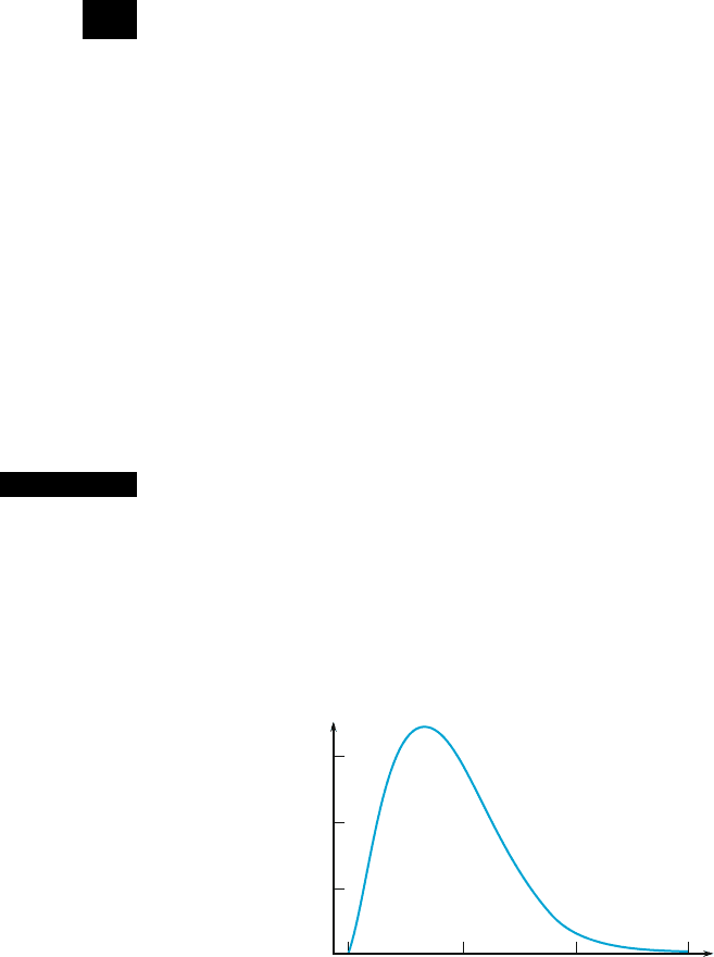
Example 6.1 Sup pose that material strength for a randomly selected specimen of a particular

type has a Weibul l distribution with parameter values a ¼ 2 (shape) and b ¼ 5

(scale). The corresponding density curve is shown in Figure 6.1. Formulas from

Section 4.5 give

m ¼ EðXÞ¼4:4311

m ¼ 4:1628 s

¼ VðXÞ¼5:365 s ¼ 2:316

The mean exceeds the median because of the distribution’s positive skew.

We used MINITAB to generate six different samples, each with n ¼ 10,

from this distribution (material strengths for six different groups of ten specimens

each). The results appear in Table 6.1, followed by the values of the sample mean,

sample median, and sample standard deviation for each samp le. Notice first that the

ten observations in any particular sample are all differ ent from those in any

other sample. Second, the six values of the sample mean are all different from

each other, as are the six values of the sample median and the six values of

the sample standard deviation. The same is true of the sample 10% trimmed

means, sample fourth spreads, and so on.

0510

.05

.10

.15

f (x)

Figure 6.1 The Weibull density curve for Example 6.1

6.1 Statistics and Their Distributions 285

Furthermore, the value of the sample mean from any particular sample can be

regarded as a point estimate (“point” because it is a single number, corresponding

to a single point on the number line) of the population mean m, whose value is

known to be 4.4311. None of the estimates from these six samples is identical to

what is being estimated. The estimates from the second and sixth samples are much

too large, whereas the fifth sample gives a substantial underestimate. Similarly,

the sample standard deviation gives a point estimate of the population standard

deviation. All six of the resulting estimates are in error by at least a small amount.

In summary, the values of the individual sample observations vary from

sample to sample, so in general the value of any quantity computed from sample

data, and the value of a sample characteristic used as an estimate of the

corresponding population characteristic, will virtually never coincide with what

is being estimated.

■

DEFINITION

A stat istic is any quantity whose value can be calculated from sample data.

Prior to obtaining data, there is uncertainty as to what value of any particula r

statistic will result. Therefore, a statistic is a random variable and will be

denoted by an uppercase letter; a lower case letter is used to represent the

calculated or observed value of the statistic.

Thus the sample mean, regarded as a statistic (before a sample has been

selected or an experiment has been carried out), is denoted by

X; the calculated

value of this statistic is



x. Similarly, S represents the sample standard deviation

thought of as a statistic, and its computed value is s. Suppose a drug is given to a

Table 6.1 Sampl es from the Weibull distribution of Example 6.1

Sample

123456

Observation

1 6.1171 5.07611 3.46710 1.55601 3.12372 8.93795

2 4.1600 6.79279 2.71938 4.56941 6.09685 3.92487

3 3.1950 4.43259 5.88129 4.79870 3.41181 8.76202

4 0.6694 8.55752 5.14915 2.49759 1.65409 7.05569

5 1.8552 6.82487 4.99635 2.33267 2.29512 2.30932

6 5.2316 7.39958 5.86887 4.01295 2.12583 5.94195

7 2.7609 2.14755 6.05918 9.08845 3.20938 6.74166

8 10.2185 8.50628 1.80119 3.25728 3.23209 1.75468

9 5.2438 5.49510 4.21994 3.70132 6.84426 4.91827

10 4.5590 4.04525 2.12934 5.50134 4.20694 7.26081

Statistic

Mean 4.401 5.928 4.229 4.132 3.620 5.761

Median 4.360 6.144 4.608 3.857 3.221 6.342

SD 2.642 2.062 1.611 2.124 1.678 2.496

286

CHAPTER 6 Statistics and Sampling Distributions

sample of patient s, another drug is given to a second sample, and the cholesterol

levels are denoted by X

, ..., X

and Y

, ..., Y

, respectively. Then the statistic

X  Y, the difference between the two sample mean cholesterol levels, may be

important.

Any statistic, being a random variable, has a probability distribution.

In particular, the sample mean

X has a probability distribution. Suppose, for

example, that n ¼ 2 components are randomly selected and the number of break-

downs while under warra nty is determined for each one. Possible values for the

sample mean number of breakdowns

X are 0 (if X

¼ X

¼ 0), .5 (if either X

¼ 0

and X

¼ 1orX

¼ 1 and X

¼ 0), 1, 1.5, .... Th e probability distribution of X

specifies Pð

X ¼ 0Þ, PðX ¼ : 5Þ and so on, from which other probabilities such as

Pð1 

X  3Þ and PðX  2:5Þ can be calculated. Similarly, if for a sample of size

n ¼ 2, the only possible values of the sample variance are 0, 12.5, and 50 (which is

the case if X

and X

can each take on only the values 40, 45, and 50), then

the probability distribution of S

gives P (S

¼ 0), P(S

¼ 12.5), and P(S

¼ 50).

The probability distribution of a statistic is sometimes referred to as its sampling

distribution to emphasize that it describes how the statistic varies in value across

all samples that might be select ed.

Random Samples

The probability distribution of any particular statistic depends not only on the

population distribution (normal, uniform, etc.) and the sample size n but also on

the method of sampling. Consider selecting a sample of size n ¼ 2 from a popula-

tion consisting of just the three values 1, 5, and 10, and suppose that the statistic of

interest is the sample variance. If sampling is done “with replacement,” then S

¼ 0

will result if X

¼ X

. However, S

cannot equal 0 if sampling is “without replace-

ment.” So P(S

¼ 0) ¼ 0 for one sampling method, and this probability is positive

for the other method. Our next definition describes a sampling method often

encountered (at least approximately) in practice.

DEFINITION

The rv’s X

, X

, ..., X

are sai d to form a (simple) random sample of size n if

1. Th e X

’s are independent rv’s.

2. Ev ery X

has the same probability distribution.

Conditions 1 and 2 can be paraphrased by saying that the X

’s are independent and

identically distributed (iid). If sampling is either with replacement or from an

infinite (conceptual) population, Conditions 1 and 2 are satisfied exactly. These

conditions will be approximately satisfied if sampling is without replacement,

yet the sample size n is much smaller than the population size N. In practice,

if n/N  .05 (at most 5% of the population is sampled), we can proceed as if

the X

’s form a random sample. The virtue of this sampling method is that the

probability distribution of any statistic can be more easily obtained than for any

other sampling method.

6.1 Statistics and Their Distributions 287