Devore J.L., Berk K.N. Modern Mathematical Statistics with Applications

Подождите немного. Документ загружается.

Example 6.7 Th e time that it takes a randomly selected rat of a certain subspecies to find its way

through a maze is a normally distributed rv with m ¼ 1.5 min and s ¼ .35 min.

Suppose five rats are selected. Let X

, ..., X

denote their times in the maze.

Assuming the X

’s to be a random sample from this normal distribution, what is the

probability that the total time T

¼ X

þ ···þ X

for the five is between 6 and

8 min? By the proposition, T

has a normal distribution with m

¼ nm ¼

5ð1:5Þ¼7:5 and variance s

¼ ns

¼ 5ð:1225Þ¼:6125, so s

¼ :783. To stan-

dardize T

, subtract m

and divide by s

Pð6  T

 8Þ¼P

6  7:5

:783

 Z 

8  7:5

:783



¼ P 1:92  Z  :64ðÞ

¼ Fð:64ÞFð1:92Þ¼:7115

Determination of the probability that the sample average time

X (a normally

distributed variable) is at most 2.0 min requires m

¼ m ¼ 1:5 and s

¼ s=

ﬃﬃﬃ

:35=

ﬃﬃﬃ

¼ :1565. Then

Pð

X  2:0Þ¼PZ

2:0  1:5

:1565



¼ PZ 3:19ðÞ¼Fð3:19Þ¼:9993

■

The Central Limit Theorem

When the X

’s are normally distributed, so is X for every sample size n. The

simulation experiment of Example 6.5 suggests that even when the population

distribution is highly nonnormal, averaging produces a distribution more bell-

shaped than the one being sampled. A reasonable conjecture is that if n is large, a

suitable normal curve will approximate the actual distribution of

X. The formal

statement of this result is the most important theorem of probability.

THEOREM

The Central Limit Theorem (CLT)

Let X

, X

, ..., X

be a random sample from a distribution with mean m and

variance s

. Then, in the limit as n !1, the standardized versions of X and

have the standard normal distribution. That is,

lim

n!1

X  m

ﬃﬃﬃ

 z



¼ PðZ  zÞ¼FðzÞ

and

lim

n!1

 nm

ﬃﬃﬃ

 z



¼ PðZ  zÞ¼FðzÞ

where Z is a standard normal rv. As an alternative to saying that the standardized

versions of

X and T

have limiting standard normal distributions, it is customary

to say that

X and T

are asymptotically normal. Thus when n is sufficiently

large,

X has approximately a normal distribution with mean m

¼ m and

variance s

¼ s

=n. Equivalently, for large n the sum T

has approximately a

normal distribution with mean m

¼ nm and variance s

¼ ns

298 CHAPTER 6 Statistics and Sampling Distributions

A partial proof of the CLT appears in the appendix to this chapter. It is shown

that, if the moment generating function exists, then the mgf of the standardized

(and T

) approaches the standard normal mgf. With the aid of an advanced

probability theorem, this implies the CLT statement about convergence of prob-

abilities.

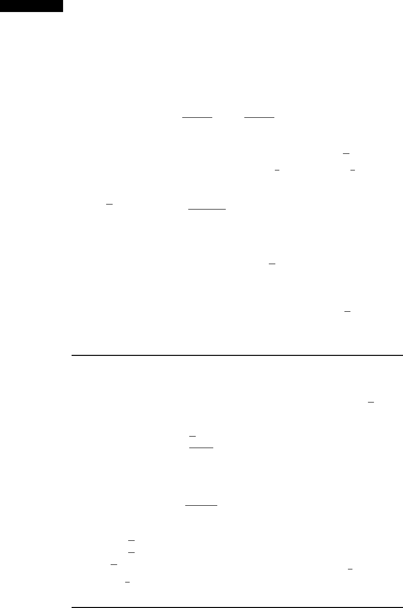
Figure 6.10 illustrates the Central Limit Theorem. According to the CLT,

when n is large and we wish to calculate a probability such as Pða 

X  bÞ, we

need only “pretend” that

X is normal, standardize it, and use the normal table. The

resulting answer will be approximately correct. The exact answer could be obtained

only by first finding the distribution of

X, so the CLT provides a truly impressive

shortcut.

Example 6.8 When a batch of a certain chemical product is prepared, the amount of a particular

impurity in the batch is a random variable with mean value 4.0 g and standard

deviation 1.5 g. If 50 batches are independently prepared, what is the (approximate)

probability that the sample average amount of impurity

X is between 3.5 and 3.8 g?

According to the rule of thumb to be stated shortly, n ¼ 50 is large enough for the

CLT to be applicable. The mean

X then has approximately a normal distribution

with mean value m

¼ 4:0 and s

¼ 1:5=

ﬃﬃﬃﬃﬃ

¼ :2121, so

Pð3:5 

X  3:8Þ¼P

3:5  4:0

:2121

 Z 

3:8  4:0

:2121



¼ Fð:94ÞFð2:36Þ¼:1645

■

Example 6.9 Sup pose the number of times a randomly selected customer of a large bank uses the

bank’s ATM during a particular period is a random variable with a mean value of

3.2 and a standard deviation of 2.4. Among 100 randomly selected customers, how

likely is it that the sample mean number of times the bank’s ATM is used exceeds 4?

Let X

denote the number of times the ith customer in the sample uses the

bank’s ATM. Notice that X

is a discrete rv, but the CLT is not limited to

continuous random variables. Also, although the fact that the standard deviation

of this nonnegative variable is quite large relative to the mean value suggests

X distribution for

small to moderate n

Population

distribution

X distribution for

large n (approximately normal)

Figure 6.10 The Central Limit Theorem illustrated

6.2 The Distribution of the Sample Mean 299

that its distribution is positively skewed, the large sample size implies that X does

have approximately a normal distribution. Using m

¼ 3:2 and s

¼ :24,

Pð

X > 4ÞPZ>

4  3:2

:24



¼ 1  Fð3:33Þ¼:0004

■

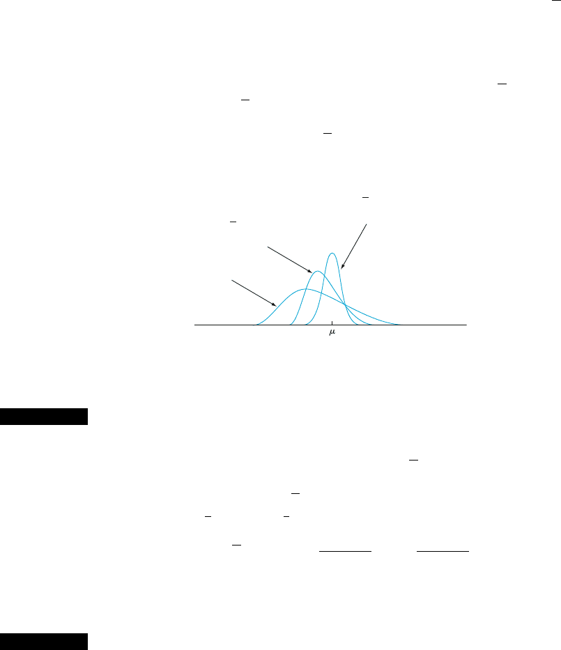
Example 6.10 Consider the distribution shown in Figure 6.11 for the amount purchased (rounded

to the nearest dollar) by a randomly select ed customer at a particular gas station

(a similar distribution for purchases in Britain (in £) appeared in the article “Da ta

Mining for Fun and Profit”, Statistical Science, 2000: 111–131; there were big

spikes at the values 10, 15, 20, 25, and 30). The distribution is obvio usly quite non-

normal.

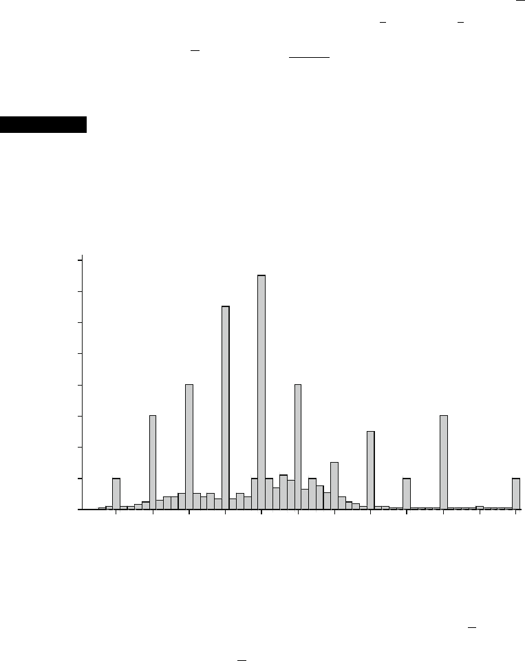
We asked MINITAB to select 1000 different samples, each consisting of

n ¼ 15 observations, and calculate the value of the sample mean

X for each one.

Figure 6.12 is a histogram of the resulting 1000 values; this is the approximate

sampling distribution of

X under the specified circumstances. This distribution is

clearly approximately normal even though the sample size is not all that large. As

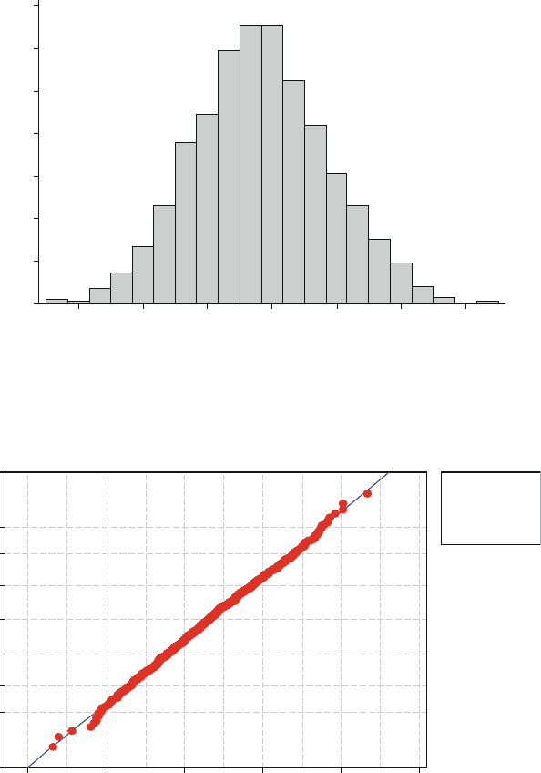
further evidence for normal ity, Figure 6.13 shows a normal probability plot of the

1000



x values; the linear pattern is very prominent. It is typically not non-normality

in the central part of the population distribution that causes the CLT to fail, but

instead very substantial skewness.

5 1015202530354045505560

0.16

0.14

0.12

0.10

0.08

0.06

0.04

0.02

0.00

probability

purchase amount

Figure 6.11 Probability distribution of

¼ amount of gasoline purchased ($)

300

CHAPTER 6 Statistics and Sampling Distributions

A practical difficulty in applying the CLT is in knowing when n is suffi-

ciently large. The problem is that the accuracy of the approximation for a particular

n depends on the shape of the original underlying distribution being sampled. If the

underlying distribution is symmetric and there is not much probability in the tails,

then the approximation will be good even for a small n, whereas if it is highly

skewed or there is a lot of probability in the tails, then a large n will be required.

For example, if the distribution is uniform on an interval, then it is symmetric with

no probability in the tails, and the normal approximation is very good for n as

0.14

0.12

0.10

0.08

0.06

0.04

0.02

0.00

18 21 24 27 30 33 36

density

mean

Figure 6.12 Approximate sampling distribution of the sample mean amount

purchased when

¼ 15 and the population distribution is as shown in Figure 6.11

99.99

0.01

15 20 25 30 35 40

percent

mean

Mean

StDev

P-Value

26.49

3.112

1000

>0.100

0.999

Figure 6.13 Normal probability plot from MINITAB of the 1000



values based on

samples of size

¼ 15 ■

6.2 The Distribution of the Sample Mean 301

small as 10. However, at the other extreme, a distribution can have such fat tails

that the mean fails to exist and the Central Limit Theorem does not apply, so no n is

big enough. We will use the following rule of thumb, which is frequently somewhat

conservative.

RULE OF

THUMB

If n > 30, the Central Limit Theorem can be used.

Of course, there are exceptions, but this rule applies to most distributions of

real data.

Other Applications of the Central Limit Theorem

The CLT can be used to justify the normal approximation to the binomial distribu-

tion discusse d in Chapter 4. Recall that a binomial variable X is the number of

successes in a binomial experiment consisting of n independent success/failure

trials with p ¼ P(S) for any particular trial. Define new rv’s X

, X

, ..., X

1 if the ith trial results in a success

0 if the ith trial results in a failure

(

ði ¼ 1; ...; nÞ

Because the trials are independent and P(S) is constant from trial to trial, the X

’s

are iid (a random sample from a Bernoulli distribution). The CLT then implies that

if n is sufficiently large, both the sum and the average of the X

’s have approxi-

mately normal distributions. When the X

’s are summed, a 1 is added for every S

that occurs and a 0 for every F, so X

þ ···þ X

¼ X ¼ T

. The sample mean of

the X

’s is X ¼ Xn

, the sample proportion of successes. That is, both X and X/n

are approximately normal when n is large. The necessary sample size for this

approximation depends on the value of p: When p is close to .5, the distribution

of each X

is reasonably symmetric (see Figure 6.14), whereas the distribution is

quite skewed when p is near 0 or 1. Using the approximation only if both np  10

and n(1 – p)  10 ensures that n is large enough to overcome any skewness in the

underlying Bernoulli distribution.

Recall from Section 4.5 that X has a lognormal distribution if ln(X) has a

normal distribut ion.

01 01

Figure 6.14 Two Bernoulli distributions: (a)

¼ .4 (reasonably symmetric);

(b)

¼ .1 (

very

skewed)

302

CHAPTER 6 Statistics and Sampling Distributions

PROPOSITION

Let X

, X

, ..., X

be a random sample from a distribution for which only

positive values are possible [P(X

> 0) ¼ 1]. Then if n is sufficiently large,

the product Y ¼ X

·····X

has approximately a lognormal distribution;

that is, ln(Y) has a normal distribution.

To verify this, note that

lnðYÞ¼ln X

ðÞþln X

ðÞþþlnðX

Since ln (Y) is a sum of independent and identically distributed rv’s [the ln(X

)’s], it

is appro ximately normal when n is large, so Y itself has approximately a lognormal

distribution. As an example of the applicability of this result, it has been argued that

the damage process in plastic flow and crack propagation is a multiplicative

process, so that variables such as percentage elongation and rupture strength have

approximately lognormal distributions.

The Law of Large Numbers

Recall the first proposition in this section: If X

, X

, ..., X

is a random sample

from a distribution with mean m and variance s

, then E ðXÞ¼m and VðXÞ¼s

What happens to

X as the number of observations becomes large? The expected

value of

X remains at m but the variance approaches zero. That is,

Vð

XÞ¼E½ð X  mÞ

! 0. We say that X converges in mean square to m because

the mean of the squared difference between

X and m goes to zero. This is one form

of the Law of Large Numbers, which says that

X ! m as n !1.

The law of large numbers should be intuitively reasonable. For example,

consider a fair die with equal probabilities for the values 1, 2, ...,6som ¼ 3.5.

After many repeated thr ows of the die x

, x

, ..., x

, we should be surprised if



x is

not close to 3.5.

Another form of convergence can be shown with the help of Chebyshev’s

inequality (Exercises 43 and 135 in Chapter 3), which states that for any random

variable Y, P(jY  mjks)  1/k

whenever k  1. In words, the p robability that

Y is at least k standard deviations away from its mean valu e is at most 1/k

;ask

increases, the probability gets closer to 0. Apply this to the mean Y ¼

X of a

random sample X

, X

, ..., X

from a distribution with mean m and variance s

Then EðYÞ¼Eð

XÞ¼m and VðYÞ¼VðXÞ¼s

, so the s in Chebyshev’s

inequality needs to be replaced by s

ﬃﬃﬃ

. Now let e be a positive number close

to 0, such as .01 or .001, and consider Pð

X  m

 eÞ, the probability that X differs

from m by at least e (at least .01, at least .001, etc.). What happens to this probability

as n !1? Setting e ¼ ks

ﬃﬃﬃ

and solving for k gives k ¼ e

ﬃﬃﬃ

. Thus

Pð

X  m

 eÞ¼P X  m



ﬃﬃﬃ



ﬃﬃﬃ





ﬃﬃﬃ



so as n gets arbitrarily large, the probability will approach 0 regardless of how

small e is. That is, for any e, the chance that

X will differ from m by at least e

6.2 The Distribution of the Sample Mean 303

decreases to 0 as the sample size increases. Because of this, statisticians say that X

converges to m in probability.

We can summarize the two forms of the Law of Large Numbers in the

following theorem.

THEOREM

If X

, X

, ..., X

is a random sample from a distribution with mean m and

variance s

, then X converges to m

a. In mean square: E

X  mðÞ½

! 0asn !1

b. In probability: P

X  m

 eðÞ!0asn !1for any e > 0

Often we do not know m so we use

X to estimate it. According to the theorem,

X will be an accurate estimator if n is large. Estimators that are close for large n are

called consistent.

Example 6.11 Let’s apply the Law of Large Numbers to the repeated flipping of a fair coin.

Intuitively, the fraction of heads should approach

as we get more and more coin

flips. For i ¼ 1, ...n, let X

¼ 1 if the ith toss is a head and ¼ 0 if it is a tail. Then

the X

’s are independent and each X

is a Bernoulli rv with m ¼ .5 and standard

deviation s ¼ .5. Furthermore, the sum X

þ X

þ ... þ X

is the total number of

heads, so

X is the fraction of heads. Thus, the fraction of heads approaches the

mean, m ¼ .5, by the Law of Large Numbers.

■

Exercises Section 6.2 (11–26)

11. The inside diameter of a randomly selected pis-

ton ring is a random variable with mean value

12 cm and standard deviation .04 cm.

a. If

X is the sample mean diameter for a random

sample of n ¼ 16 rings, where is the sampling

distribution of

X centered, and what is the

standard deviation of the

X distribution?

b. Answer the questions posed in part (a) for a

sample size of n ¼ 64 rings.

c. For which of the two random samples, the one

of part (a) or the one of part (b), is

X more

likely to be within .01 cm of 12 cm? Explain

your reasoning.

12. Refer to Exercise 11. Suppose the distribution of

diameter is normal.

a. Calculate Pð11:99 

X  12:01Þwhen n ¼ 16.

b. How likely is it that the sample mean diame-

ter exceeds 12.01 when n ¼ 25?

13. The National Health Statistics Reports dated Oct.

22, 2008 stated that for a sample size of 277 18-

year-old American males, the sample mean waist

circumference was 86.3 cm. A somewhat compli-

cated method was used to estimate various popula-

tion percentiles, resulting in the following values:

5th 10th 25th 50th 75th 90th 95th

69.6 70.9 75.2 81.3 95.4 107.1 116.4

a. Is it plausible that the waist size distribution is

at least approximately normal? Explain your

reasoning. If your answer is no, conjecture the

shape of the population distribution.

b. Suppose that the population mean waist size

is 85 cm and that the population standard

deviation is 15 cm. How likely is it that a

random sample of 277 individuals will result

in a sample mean waist size of at least 86.3 cm?

c. Referring back to (b), suppose now that the

population mean waist size is 82 cm (closer to

the median than the mean). Now what is the

(approximate) probability that the sample

mean will be at least 86.3? In light of this

calculation, do you think that 82 is a reason-

able value for m?

304

CHAPTER 6 Statistics and Sampling Distributions

14. There are 40 students in an elementary statistics

class. On the basis of years of experience, the

instructor knows that the time needed to grade a

randomly chosen first examination paper is a

random variable with an expected value of

6 min and a standard deviation of 6 min.

a. If grading times are independent and the

instructor begins grading at 6:50 p.m. and

grades continuously, what is the (approxi-

mate) probability that he is through grading

before the 11:00 p.m. TV news begins?

b. If the sports report begins at 11:10, what is the

probability that he misses part of the report if

he waits until grading is done before turning

on the TV?

15. The tip percentage at a restaurant has a mean

value of 18% and a standard deviation of 6%.

a. What is the approximate probability that the

sample mean tip percentage for a random

sample of 40 bills is between 16% and 19%?

b. If the sample size had been 15 rather than 40,

could the probability requested in part (a) be

calculated from the given information?

16. The time taken by a randomly selected applicant

for a mortgage to fill out a certain form has a

normal distribution with mean value 10 min and

standard deviation 2 min. If five individuals fill

out a form on 1 day and six on another, what is

the probability that the sample average amount

of time taken on each day is at most 11 min?

17. The lifetime of a type of battery is normally

distributed with mean value 10 h and standard

deviation 1 h. There are four batteries in a pack-

age. What lifetime value is such that the total

lifetime of all batteries in a package exceeds that

value for only 5% of all packages?

18. Let X represent the amount of gasoline (gallons)

purchased by a randomly selected customer

at a gas station. Suppose that the mean value

and standard deviation of X are 11.5 and 4.0,

respectively.

a. In a sample of 50 randomly selected custo-

mers, what is the approximate probability that

the sample mean amount purchased is at least

12 gallons?

b. In a sample of 50 randomly selected custo-

mers, what is the approximate probability that

the total amount of gasoline purchased is at

most 600 gallons.

c. What is the approximate value of the 95th

percentile for the total amount purchased by

50 randomly selected customers.

19. Suppose the sediment density (g/cm) of a ran-

domly selected specimen from a region is nor-

mally distributed with mean 2.65 and standard

deviation .85 (suggested in “Modeling Sediment

and Water Column Interactions for Hydrophobic

Pollutants,” Water Res., 1984: 1169–1174).

a. If a random sample of 25 specimens is selected,

what is the probability that the sample average

sediment density is at most 3.00? Between 2.65

and 3.00?

b. How large a sample size would be required to

ensure that the first probability in part (a) is at

least .99?

20. The first assignment in a statistical computing class

involves running a short program. If past experience

indicates that 40% of all students will make no

programming errors, compute the (approximate)

probability that in a class of 50 students

a. At least 25 will make no errors [Hint: Normal

approximation to the binomial]

b. Between 15 and 25 (inclusive) will make no

errors

21. The number of parking tickets issued in a certain

city on any given weekday has a Poisson distribu-

tion with parameter l ¼ 50. What is the approxi-

mate probability that

a. Between 35 and 70 tickets are given out on a

particular day? [Hint:Whenl is large, a Poisson

rv has approximately a normal distribution.]

The total number of tickets given out during a

5-day week is between 225 and 275?

22. Suppose the distribution of the time X (in hours)

spent by students at a certain university on a partic-

ular project is gamma with parameters a ¼ 50 and

b ¼ 2. Because a is large, it can be shown that X has

approximately a normal distribution. Use this fact to

compute the probability that a randomly selected

student spends at most 125 h on the project.

23. The Central Limit Theorem says that

X is approx-

imately normal if the sample size is large. More

specifically, the theorem states that the standar-

dized

X has a limiting standard normal distribu-

tion. That is, ð

X  mÞ=ðs=

ﬃﬃﬃ

Þ has a distribution

approaching the standard normal. Can you recon-

cile this with the Law of Large Numbers? If the

standardized

X is approximately standard normal,

then what about

X itself?

24. Assume a sequence of independent trials, each

with probability p of success. Use the Law of

Large Numbers to show that the proportion of suc-

cesses approaches p as the number of trials becomes

large.

6.2 The Distribution of the Sample Mean 305

25. Let Y

be the largest order statistic in a sample of

size n from the uniform distribution on [0, y].

Show that Y

converges in probability to y, that

is, that PðjY

 yjeÞ!0asn approaches 1.

[Hint: The pdf of the largest order statistic appears

in Section 5.5, so the relevant probability can be

obtained by integration (Chebyshev’s inequality is

not needed).]

26. A friend commutes by bus to and from work

6 days/week. Suppose that waiting time is uni-

formly distributed between 0 and 10 min, and

that waiting times going and returning on various

days are independent of each other. What is the

approximate probability that total waiting time

for an entire week is at most 75 min? [Hint:

Carry out a simulation experiment using statistical

software to investigate the sampling distribu-

tion of T

under these circumstances. The idea of

this problem is that even for an n as small as 12,

and X should be approximately normal when

the parent distribution is uniform. What do

you think?]

6.3

The Mean, Variance, and MGF

for Several Variables

The sample mean X and sample total T

are special cases of a type of random

variable that arises very frequently in statistical applications.

DEFINITION

Given a collection of n random variables X

, X

, ..., X

and n numerical

constants a

, ..., a

, the rv

Y ¼ a

þþa

i¼1

ð6:6Þ

is called a linear combination of the X

’s.

Taking a

¼ a

¼ ···¼ a

¼ 1 gives Y ¼ X

þ ···þ X

¼ T

, and

¼ a

¼¼a

yields Y ¼

þþ

þþX

ðÞ¼

¼ X. Notice that we are not requiring the X

’s to be independent or identically

distributed. All the X

’s could have different distributions and therefore differ ent

mean values and variances. We first consider the expected value and variance of a

linear combination.

PROPOSITION

Let X

, X

, ..., X

have mean values m

, ..., m

, respectively, and variances

; ...; s

, respective ly.

1. Whether or not the X

’s are independent,

Eða

þþa

Þ¼a

EðX

Þþþa

EðX

¼ a

þþa

ð6:7Þ

306 CHAPTER 6 Statistics and Sampling Distributions

2. If X

, ..., X

are independent,

Vða

þþa

Þ¼a

VðX

Þþþa

VðX

¼ a

þþa

ð6:8Þ

and

þþa

ﬃﬃﬃﬃﬃﬃﬃﬃﬃﬃﬃﬃﬃﬃﬃﬃﬃﬃﬃﬃﬃﬃﬃﬃﬃﬃﬃﬃﬃﬃﬃﬃﬃﬃﬃ

þþa

ð6:9Þ

3. For any X

, X

, ..., X

Vða

þþa

Þ¼

i¼1

j¼1

covðX

; X

Þð6:10Þ

Proofs are sketched out later in the section. A paraphrase of (6.7) is that the

expected value of a linear combination is the same linear combination of the

expected values—for example, E(2X

þ 5X

) ¼ 2m

þ 5m

. The result (6.8)in

Statement 2 is a special case of ( 6.10) in Statement 3; when the X

’s are indepen-

dent, Cov(X

, X

) ¼ 0 for i 6¼ j and ¼ V(X

) for i ¼ j (this simplification actually

occurs when the X

’s are uncorrelated, a weaker condition than independence).

Specializing to the case of a random sample (X

’s iid) with a

¼ 1/n for every i

gives E ð

XÞ¼m and VðXÞ¼s

, as discussed in Section 6.2. A similar comment

applies to the rules for T

Example 6.12 A gas station sells three grades of gasolin e: regular, plus, and premium. These are

priced at $3.50, $3.65, and $3.80 per gallon, respectively. Let X

, and X

denote

the amounts of these grades purchased (gallons) on a particular day. Suppose the

’s are independent with m

¼ 1000, m

¼ 500, m

¼ 300, s

¼ 100, s

¼ 80,

and s

¼ 50. The revenue from sales is Y ¼ 3.5X

þ 3.65X

þ 3.8X

, and

EðYÞ¼3:5m

þ 3:65m

þ 3:8m

¼ $6465

VðYÞ¼3:5

þ 3:65

þ 3:8

¼ 243; 864

ﬃﬃﬃﬃﬃﬃﬃﬃﬃﬃﬃﬃﬃﬃﬃﬃﬃ

243; 864

¼ $493:83

■

Example 6.13 The results of the previous proposition allow for a straightforward derivation of

the mean and variance of a hypergeometric rv, which were given without proof in

Section 3.6. Recall that the distribution is defined in terms of a population with N

items, of which M are successes and N–Mare failures. A sample of size n is drawn,

of which X are successes. It is equivalent to view this as random arrangement of all

N items, followed by selection of the first n. Let X

be 1 if the ith item is a success

and 0 if it is a failure, i ¼ 1, 2, ..., N. Then

X ¼ X

þ X

þ þX

According to the proposition, we can find the mean and variance of X if

we can find the means, variances, and covariances of the terms in the sum.

6.3 The Mean, Variance, and MGF for Several Variables 307