Devore J.L., Berk K.N. Modern Mathematical Statistics with Applications

Подождите немного. Документ загружается.

The model is additive if and only if all g

’s ¼ 0. The g

’s are referred to as the

interaction parameters. The a

’s are called the main effects for factor A, and the

’s are the main effects for factor B. Although there are I a

’s, J b

’s, and IJ g

’s in

addition to m, the conditions Sa

¼ 0, Sb

¼ 0, S

¼ 0 for any i, and S

¼ 0

for any j [all by virtue of (11.15) and ( 11.16)], imply that only IJ of these new

parameters are independently determined: m, I–1 of the a

’s, J–1 of the b

’s, and

(I–1)(J–1) of the g

’s.

There are now three sets of hypotheses that will be considered:

0AB

: g

¼ 0 for all i; j versus H

aAB

: at least one g

6¼ 0

: a

¼ a

¼¼a

¼ 0 versus H

: at least one a

6¼ 0

: b

¼ b

¼¼b

¼ 0 versus H

: at least one b

6¼ 0

The no-interaction hypothesis H

0AB

is usually tested first. If H

0AB

is not rejected,

then the other two hypotheses can be tested to see whether the main effects are

significant. But once H

0AB

is rejected, we believe that the effect of factor A at any

particular level depends on the level of B (and vice versa). It then does not make

sense to test H

or H

. In this context a picture similar to that of Figure 11.7(b) is

helpful in visualizing the way the factors interact. Here the cell means are used

instead of x

; this type of graph is sometimes called an interaction plot.

In case of interaction, it may be appropriate to do a one-way ANOVA to

compare levels of A separately for each level of B. For example, suppose factor A

involves four kinds of glue, factor B involves three types of material, the response is

strength of the glue joint, and the strength rankings of the glues clearly depend on

which material is being glued. In this situation with interaction, it makes sense to do

three separate one-way ANOVA analyses, one for each material.

Notation, Model, and Analysis

We now use triple subscripts for both random variables and observed values, with

ijk

and x

ijk

referring to the kth observation (replication) when factor A is at level i

and factor B is at level j. The model is then

ijk

¼ m þ a

þ b

þ g

þ e

ijk

i ¼ 1; :::; I; j ¼ 1; :::; J; k ¼ 1; :::; K

ð11:18Þ

where the e

ijk

’s are independent and normally distributed, each with mean

0 and variance s

Again a dot in place of a subscript means that we have summed over all

values of that subscript, whereas a horizontal bar denotes averaging. Thus X

ij·

is the

total of all K observations made for factor A at level i and factor B at level j [all

observations in the (i, j)th cell], and

ij

is the average of these K observations.

598 CHAPTER 11 The Analysis of Variance

Example 11.16 Three different varieties of tomato (Harvester, Ife No. 1, and Pusa Early Dwarf) and

four different plant densities (10, 20, 30, and 40 thousand plants per hectare) are

being considered for planting in a particular region. To see whether either variety or

plant density affects yield, each combination of variety and plant density is used in

three different plots, resulting in the data on yields in Table 11.8 (based on the

article “Effects of Plant Density on Tomato Yields in Western Nigeria,” Exper.

Agric., 1976: 43–47).

Here, I ¼ 3, J ¼ 4, and K ¼ 3, for a total of IJK ¼ 36 observations

■

To test the hypotheses of interest, we again define sums of squares and

present computing formulas:

SST ¼

ðX

ijk

 X



ijk



IJK



df ¼ IJK  1

SSE ¼

ðX

ijk

 X

ij

ijk



ij

df ¼ IJðK  1Þ

SSA ¼

ðX

i

 X



i



IJK



df ¼ I  1

SSB ¼

ðX

j

 X



j



IJK



df ¼ J  1

SSAB ¼

ðX

ij

 X

i

 X

j

þ X



df ¼ðI  1ÞðJ  1Þ

The fundamental identity

SST ¼ SSA þ SSB þ SSAB þ SSE

implies that the interaction sum of squares SSAB can be obtained by

subtraction.

Table 11.8 Yield data for Example 11.16

Planting Density

Variety 10,000 20,000 30,000 40,000 x

i



i

H 10.5 9.2 7.9 12.8 11.2 13.3 12.1 12.6 14.0 10.8 9.1 12.5 136.0 11.33

Ife 8.1 8.6 10.1 12.7 13.7 11.5 14.4 15.4 13.7 11.3 12.5 14.5 146.5 12.21

P 16.1 15.3 17.5 16.6 19.2 18.5 20.8 18.0 21.0 18.4 18.9 17.2 217.5 18.13

.j.

103.3 129.5 142.0 125.2 500.00



j

11.48 14.39 15.78 13.91 13.89

11.5 Two-Factor ANOVA with K

> 1 599

The computing formulas are all obtained by expanding the squared expres-

sions and summing. The fundamental identity is obtained by squaring and summing

an expression similar to Equation (11.2).

Total variation is thus partitioned into four pieces: unexplained (SSE—which

would be present whether or not any of the three null hypotheses was true) and three

pieces that may be explained by the truth or falsity of the three H

’s. Each of four

mean squares is defined by MS ¼ SS/df. The expected mean squares suggest that

each set of hypotheses should be tested using the appropriate ratio of mean squares

with MSE in the denominator:

E(MSE) ¼ s

E(MSA) ¼ s

I  1

i¼1

E(MSB) ¼ s

J  1

j¼1

E(MSAB) ¼ s

ðI  1ÞðJ  1Þ

i¼1

j¼1

Each of the three mean square ratios can be shown to have an F distribution

when the associated H

is true, which yields the followi ng level a test procedures.

Hypotheses Test Statistic Value Rejection Region

versus H

MSA

MSE

 F

;I1;IJðK1Þ

versus H

MSB

MSE

 F

;J1;IJð K1Þ

0AB

versus H

aAB

MSAB

MSE

 F

;ðI1ÞðJ1Þ;IJðK1Þ

As before, the results of the analysis are summarized in an ANOVA table.

Example 11.17

(Example 11.16

continued)

From the given data, x



¼ 500

¼ 250;000.

ijk

¼10:5

þ 9:2

þþ18:9

þ 17:2

¼ 7404:80

i

¼136:0

þ 146:5

þ 217:5

¼ 87;264:50

and

j

¼ 63;280:18

The cell totals (x

ij.

’s) are

10,000 20,000 30,000 40,000

H 27.6 37.3 38.7 32.4

Ife 26.8 37.9 43.5 38.3

P 48.9 54.3 59.8 54.5

600

CHAPTER 11 The Analysis of Variance

from which

ij

¼ 27:6

þþ54:5

¼ 22;100:28. Then

SST ¼ 7404:80 

ð250;000Þ¼7404:80  6944:44 ¼ 460:36

SSA ¼

ð87;264:50Þ6944:44 ¼ 327:60

SSB ¼

ð63;280:18Þ6944:44 ¼ 86:69

SSE ¼ 7404:80 

ð22;100:28Þ¼38:04

and

SSAB ¼ 460:36  327:60  86:69  38:04 ¼ 8:03

Table 11.9 summarizes the computation.

Since F

.01,6,24

¼ 3.67 and f

¼ .84 is not  3.67, H

0AB

cannot be rejected at level

.01, so we conclude that the interaction effects are not significant. Now the presence

or absence of main effects can be investigated. Since F

.01,2,24

¼ 5.61 and f

¼ 103.02

 5.61, H

is rejected at level .01 in favor of the conclusion that different varieties

do affect the true average yields. Similarly, f

¼ 18.18  4.72 ¼ F

.01,3,24

,sowe

conclude that true average yield also depends on plant density.

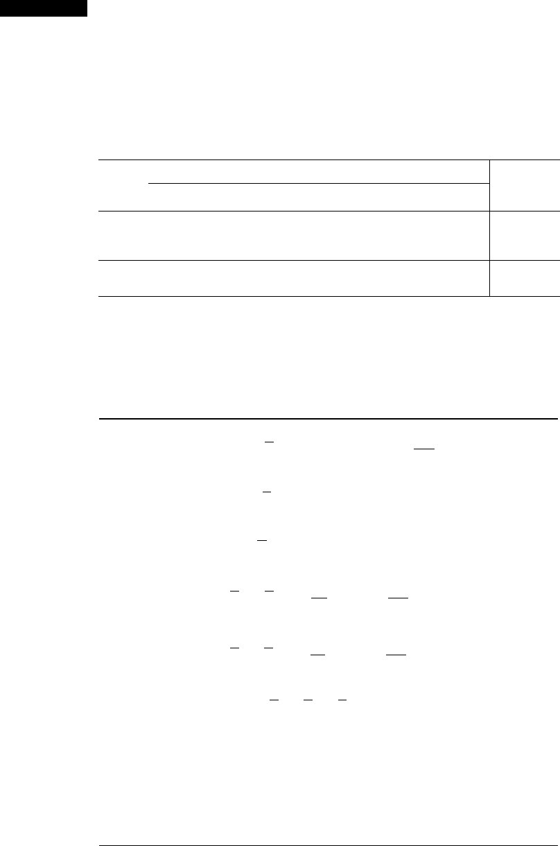
Figure 11.11 shows the interaction plot. Notice the nearly parallel lines for

the three tomato varieties, in agreement with the F test showing no significant

interaction. The yield for Pusa Early Dwarf appears to be significantly above the

yields for the other two varieties, and this is in accord with the highly significant F

for varieties. Furthermore, all three varieties show the same pattern in which yield

increases as the density goes up, but decreases beyond 30,000 per hect are. This

suggests that planting more seed will increase the yield, but eventually overcrowd-

ing causes the yield to drop.

In this example one of the two factors is quantitative, and this is naturally the

factor used for the horizontal axis in the interaction plot. In case both of the factors

are quantitative, the choice for the horizontal axis would be arbitrary, but a case can

be made for two plots to try it both ways. Indeed, MINITAB has an option to allow

both plots to be included in the same graph.

Table 11.9 ANOVA table for Example 11.17

Source of Variation df Sum of Squares Mean Square f

Varieties 2 327.60 163.8 f

¼ 103.02

Density 3 86.69 28.9 f

¼ 18.18

Interaction 6 8.03 1.34 f

¼ .84

Error 24 38.04 1.59

Total 35 460.36

11.5 Two-Factor ANOVA with K

> 1 601

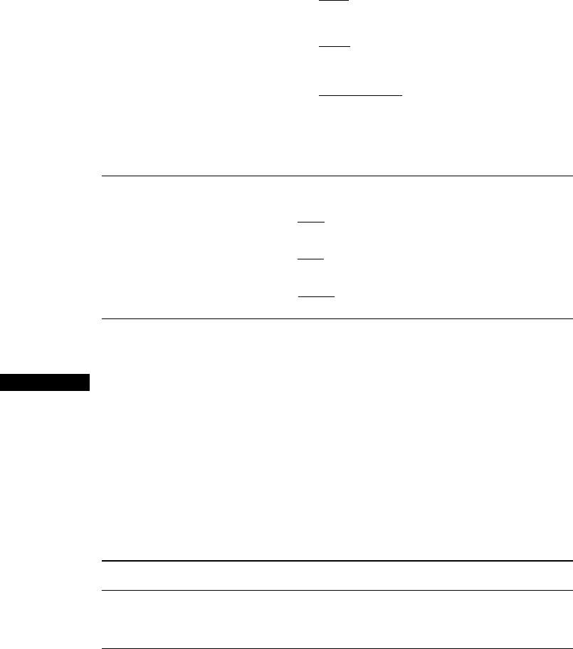
To check the normality and constant variance assumptions we can make plots

similar to those of Section 11.4. Define the predicted values (fitted values) to be the

cell means,

ijk



ij

, so the residuals, the differences between the observations and

predicted values, are x

ijk





ij

. The normal plot of the residuals is Figure 11.12(a),

and the plot of the residuals against the fitted values is Figure 11.12(b). The normal

plot is sufficiently straight that there should be no concern about the normality

assumption. The plot of residuals against predicted values has a fairly uniform

vertical spread, so there is no cause for concern about the constant variance

assumption.

10000 20000 30000 40000

Density

Mean

Variety

H Ife P

Figure 11.11 Interaction plot for the tomato yield data

0−3 −2 −1

Residual

Normal Probability Plot of the Residuals

(response is Yield)

10 12 14 16 18 20

Fitted Value

−1

−2

Residuals Versus the Fitted Values

(response is Yield)

Percent

Residual

Figure 11.12 Plots from MINITAB to verify assumptions for Example 11.17 ■

602

CHAPTER 11 The Analysis of Variance

Multiple Comparisons

When the no-interaction hypothesis H

0AB

is not rejected and at least one of the two

main-effect null hypotheses is rejected, Tukey’s method can be used to identify

significant differences in levels. To identify differences among the a

’s when H

is rejected:

1. Obtain Q

a,I,IJ(K1)

, where the second subscript I identifies the number of levels

being compared and the third subscript refers to the number of degrees of

freedom for error.

2. Compute w ¼ Q

ﬃﬃﬃﬃﬃﬃﬃﬃﬃﬃﬃﬃﬃﬃﬃﬃﬃﬃ

MSE=JK

, where JK is the number o f observations averaged

to obtain each of the



i

’s compared in step 3.

3. Or der the



i

’s from smallest to largest and, as before, underscore all pairs that

differ by less than w. Pairs not underscor ed correspond to significantly different

levels of factor A.

To identify different levels of factor B when H

is rejected, replace the second

subscript in Q by J, replace JK by IK in w, and replace



i



j

Example 11.18

(Example 11.17

continued)

For factor A (varieties), I ¼ 3, so with a ¼ .01 and IJ( K –1)¼ 24, Q

.01,3,24

4.55. Then w ¼ 4:55

ﬃﬃﬃﬃﬃﬃﬃﬃﬃﬃﬃﬃﬃﬃﬃﬃ

1:59=12

¼ 1.66, so ordering and underscoring gives



1



2



3

11.33 12.21 18.13

The Harvester and Ife varieties do not differ significantly from each other in effect

on true average yield, but both differ from the Pusa variety.

For factor B (density), J ¼ 4soQ

.01,4,24

¼ 4.91 and w ¼4:91

ﬃﬃﬃﬃﬃﬃﬃﬃﬃﬃﬃﬃﬃﬃ

1:59=9

¼ 2:06



1



4



2



3

11.48 13.91 14.39 15.78

Thus with experimentwise error rate .01, which is quite conservative, only the

lowest density differs significantly from all others. Even with a ¼ .05 (so that

w ¼ 1.64), densities 2 and 3 cannot b e judged significantly different from each

other in their effect on yield.

■

Models with Mixed and Random Effects

In some situations, the levels of either factor may have been chosen from a large

population of possible levels, so that the effect s contributed by the factor are

random rather than fixed. As in Section 11.4, if both factors contribute random

effects, the mode l is referred to as a random effects model, whereas if one factor is

fixed and the other is random, a mixed effects model results. We will now consider

the analysis for a mixed effects model in which factor A (rows) is the fixed factor

and factor B (columns) is the random factor. When either factor is random,

interaction effects will also be random. The case in which both factors are random

is dealt with in Exercise 57. The mixed effects model is

11.5 Two-Factor ANOVA with K

> 1 603

¼m þ a

þ B

þ G

þ e

ijk

i ¼1; ...; I; j ¼ 1; ...; J; k ¼ 1; ...; K

Here m and a

’s are constants with Sa

¼ 0 and the B

’s, G

’s, and e

ijk

’s are

independent, normally distributed random variables with expected value 0 and

variances s

, s

, and s

, respectively.

: a

¼¼a

¼ 0 versus H

: at least one a

6¼ 0

: s

¼ 0 versus H

: s

> 0

: s

¼ 0 versus H

: s

> 0

It is customary to test H

and H

only if the no-interaction hypothesis H

cannot

be rejected.

The relevant sums o f squares and mean squares needed for the test procedures

are defined and computed exactly as in the fixed effects case. The expected mean

squares for the mixed model are

E MSEðÞ¼s

E MSAðÞ¼s

þ Ks

I  1

E MSBðÞ¼s

þ Ks

þ IKs

and

E MSA BðÞ¼s

þ Ks

Thus, to test the no-i nteraction hypothesis, the ratio f

¼ MSAB/MSE is again

appropriate, with H

rejected if f

 F

;ðI 1ÞðJ1Þ;IJðK1Þ

. However, for testing

versus H

, the expected mean squares suggest that although the numerator of

the F ratio should still be MSA, the denominator should be MS AB rather than MSE.

MSAB is also the denominator of the F ratio for testing H

This is referred to as an “unrestricted” model. An alternative “restricted” model requires that S

¼ 0

(so the G

’s are no longer independent). Expected mean squares and F ratios appropriate for testing

certain hypotheses depend on the choice of model. Minitab’s default option gives output for the

unrestricted model.

604 CHAPTER 11 The Analysis of Variance

For testing H

versus H

(factors A fixed, B random) , the test statistic value

is f

¼ MSA/MSAB, and the rejection region is f

 F

;I1;ðI1ÞðJ1Þ

. The

test of H

versus H

utilizes f

¼ MSB/MSAB, and the rejection region is

 F

;J1;ðI1ÞðJ1Þ

Example 11.19 A process engi neer has identified two potential causes of electric motor vibration,

the material used for the motor casing (fa ctor A) and the supply source of bearings

used in the motor (factor B). The accompanying data on the amount of vibration

(microns) resulted from an experiment in which motors with casings made of steel,

aluminum, and plastic were constructed using bearings supplied by five randomly

selected sources.

Supply source

Material 12345

Steel 13.1 13.2 16.3 15.8 13.7 14.3 15.7 15.8 13.5 12.5

Aluminum 15.0 14.8 15.7 16.4 13.9 14.3 13.7 14.2 13.4 13.8

Plastic 14.0 14.3 17.2 16.7 12.4 12.3 14.4 13.9 13.2 13.1

Only the three casing materials used in the experiment are under consideration for

use in production, so factor A is fixed. However, the five supply sources were

randomly selected from a much larger population, so factor B is random. The

relevant null hypotheses are

: a

¼ a

¼ 0 H

: s

¼ 0 H

: s

¼ 0

MINITAB outpu t appears in Figure 11.13 .

Factor Type Levels Values

casmater fixed 3 1 2 3

random 5 1 2 3 4 5

DF SS MS F P

casmater 2 0.7047 0.3523 0.24 0.790

source 4 36.6747 9.1687 6.32 0.013

8 11.6053 1.4507 13.03 0.000

Error 15 1.6700 0.1113

Total 29 50.6547

Source Variance Error Expected Mean Square for Each Term

component term (using unrestricted model)

1 casmater 3 (4) + 2(3)

2(3)

3(4) + +

4 (4) +

(4)

source

Source

casmater*source

Q[1]

2 source

1.2863

6(2)

3 casmater*source 0.6697

4 Error

0.1113

Figure 11.13 Output from MINITAB’s balanced ANOVA option for the data of

Example 11.19

11.5 Two-Factor ANOVA with K

> 1 605

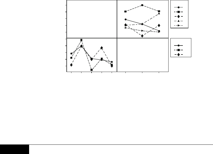
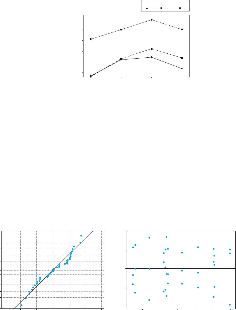
The printed 0.000 P-value for interaction means that it is less than .0005 (the

actual value is .000018). To interpret the significant interaction we use the interac-

tion plot, Figure 11.14, which has both versions, one with source on the x-axis and

one with material on the x-axis. Interaction is evident, because the best material (the

one with the least vibration) depends strongly on source. For source 1 the best

material is steel, for source 3 the best material is plastic, and for source 4 the best

material is aluminum. Because of this interaction, we ordinarily would not interpret

the main effects, but one cannot help noticing that there is strong dependence of

vibration on source. Source 2 is bad for all three materials and source 3 is pretty

good for all three materials. When one-way ANOVA analyses are done to compare

the five sources for each of the three materials, all three show highly significant

differences. This is consistent with the P-value of 0.013 for source in Figure 11.13.

We can conclude that, although the interaction causes the best material to depend

on the source, the source also makes a difference of its own.

When at least two of the K

’s are unequal, the ANOVA computations are

much more complex than for the case K

¼ K, and there are no nice formulas for

the appropriate test statistics. One of the chapter references can be consulted for

more information.

Exercises Section 11.5 (49–57)

49. In an experiment to assess the effects of curing

time (factor A) and type of mix (factor B) on the

compressive strength of hardened cement cubes,

three different curing times were used in combi-

nation with four different mixes, with three obser-

vations obtained for each of the 12 curing

time–mix combinations. The resulting sums of

squares were computed to be SSA ¼ 30,763.0,

SSB ¼ 34,185.6, SSE ¼ 97,436.8, and SST

¼ 205,966.6.

a. Construct an ANOVA table.

b. Test at level .05 the null hypothesis H

0AB

: all

’s ¼ 0 (no interaction of factors) against

0AB

: at least one g

6¼ 0.

1234

APS

Interaction Plot(data means)for vibration

Source

Material

Source

Material

Fig.11.14 MINITAB interaction plot for the data of Example 11.19 ■

606

CHAPTER 11 The Analysis of Variance

c. Test at level .05 the null hypothesis H

: a

¼ a

¼ 0 (factor A main effects are absent)

against H

: at least one a

6¼ 0.

d. Test H

: b

¼ b

¼ 0 versus H

at least one b

6¼ 0 using a level .05 test.

e. The values of the



i

’s were



1

4010:88;



2

¼ 4029:10; and



3

¼ 3960:02.

Use Tukey’s procedure to investigate signifi-

cant differences among the three curing times.

50. The article “Towards Improving the Properties of

Plaster Moulds and Castings” (J. Engrg. Manuf.,

1991: 265–269) describes several ANOVAs car-

ried out to study how the amount of carbon fiber

and sand additions affect various characteristics of

the molding process. Here we give data on casting

hardness and on wet-mold strength.

Sand

Addition

(%)

Carbon

Fiber

Addition

(%)

Casting

Hardness

Wet-

Mold

Strength

0 0 61.0 34.0

0 0 63.0 16.0

15 0 67.0 36.0

15 0 69.0 19.0

30 0 65.0 28.0

30 0 74.0 17.0

0 .25 69.0 49.0

0 .25 69.0 48.0

15 .25 69.0 43.0

15 .25 74.0 29.0

30 .25 74.0 31.0

30 .25 72.0 24.0

0 .50 67.0 55.0

0 .50 69.0 60.0

15 .50 69.0 45.0

15 .50 74.0 43.0

30 .50 74.0 22.0

30 .50 74.0 48.0

a. An ANOVA for wet-mold strength gives

SSSand ¼ 705, SSFiber ¼ 1278, SSE ¼ 843,

and SST ¼ 3105. Test for the presence of any

effects using a ¼ .05.

b. Carry out an ANOVA on the casting hardness

observations using a ¼ .05.

c. Make an interaction plot with sand percentage

on the horizontal axis, and discuss the results of

part (b) in terms of what the plot shows.

51. The accompanying data resulted from an

experiment to investigate whether yield from a

chemical process depended either on the formula-

tion of a particular input or on mixer speed.

Speed

60 70 80

189.7 185.1 189.0

1 188.6 179.4 193.0

Formulation 190.1 177.3 191.1

165.1 161.7 163.3

2 165.9 159.8 166.6

167.6 161.6 170.3

A statistical computer package gave SS(Form) ¼

2253.44, SS(Speed) ¼ 230.81, SS(Form*Speed)

¼ 18.58, and SSE ¼ 71.87.

a. Does there appear to be interaction between the

factors?

b. Does yield appear to depend on either formu-

lation or speed?

c. Calculate estimates of the main effects.

d. Verify that the residuals are 0.23,0.87, 0.63,

4.50,1.20,3.30,2.03,1.97,0.07,1.10,

0.30,1.40,0 .67,1.23,0.57,3.43,0.13,

3.57.

e. Construct a normal plot from the residuals

given in part (d). Do the e

ijk

’s appear to be

normally distributed?

f. Plot the residuals against the predicted values

(cell means) to see if the population variance

appears reasonably constant.

52. In an experiment to investigate the effect of “cement

factor” (number of sacks of cement per cubic yard)

on flexural strength of the resulting concrete (“Stud-

ies of Flexural Strength of Concrete. Part 3: Effects

of Variation in Testing Procedure,” Proceedings

ASTM, 1957: 1127–1139), I ¼ 3 different factor

values were used, J ¼ 5differentbatchesofcement

were selected, and K ¼ 2 beams were cast from

each cement factor/batch combination. Summary

values include

PPP

ijk

¼ 12;280;103,

ij

¼ 24;529;699,

i

¼ 122;380;901,

j

¼ 73;427;483, and x



¼ 19;143.

a. Construct the ANOVA table.

b. Assuming a mixed model with cement factor

(A) fixed and batches (B) random, test the three

pairs of hypotheses of interest at level .05.

53. A study was carried out to compare the writing

lifetimes of four premium brands of pens. It was

thought that the writing surface might affect life-

time, so three different surfaces were randomly

selected. A writing machine was used to ensure

that conditions were otherwise homogeneous

11.5 Two-Factor ANOVA with K

> 1 607