Devore J.L., Berk K.N. Modern Mathematical Statistics with Applications

Подождите немного. Документ загружается.

Thus x ¼ 4908=8 ¼ 613 :5, y ¼ 22:7=8 ¼ 2:838, and

15;441:4 ð4908 Þð22:7Þ=8

3;190;248 ð4908Þ

1514:95

179;190

¼ :00845443  :00845

¼2:838 ð:00845443Þð613:5Þ¼2:349

We estimate that the expected change in tree mass associated with a 1-part-per-

million increase in CO

concentration is .00845. The equation of the estimated

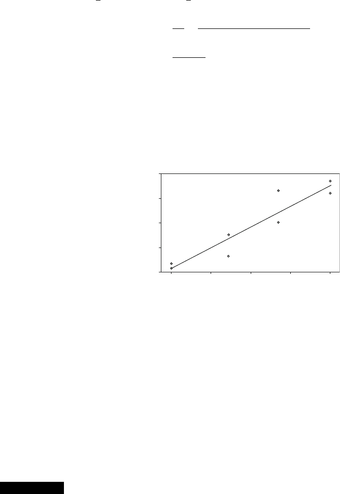
regression line (least squares line) is then y ¼2.35 + .00845x. Figure 12.10,

generated by the statistical computer package R, shows that the least squares line

provides an excellent summary of the relationship between the two variables.

The estimated regression line can immediately be used for two different pur-

poses. For a fixed x value x



;



(the height of the line above x*) gives either (1)

a point estimate of the expected value of Y when x ¼ x* or (2) a point prediction of the

Y value that will result from a single new observation made at x ¼ x*.

The least squares line should not be used to make a prediction for an x value

much beyond the range of the data, such as x ¼ 250 or x ¼ 1000 in Example 12.5.

The danger of extrapolation is that the fitted relationship (a line here) may not be

valid for such x values. (In the foregoing example, x ¼ 250 gives

y ¼:235, a

patently ridiculous value of mass, but extrapolation will not always result in such

inconsistencies.)

Example 12.6 Refer to the tree-mass-CO

data in the previous example. With a little extrapola-

tion, a point estimate for true average mass for all specimens with CO

concentra-

tion 365 is

Y365

ð365Þ¼2:35 þ :00845ð365Þ¼:73

With a little more extrapolation, a point estimate for true average mass for all

specimens with CO

concentration 315 is

Y315

ð315Þ¼2:35 þ :00845ð315Þ¼:31

510410 610 710 810

CO2

mass

Figure 12.10 A scatter plot of the data in Example 12.5 with the least squares

line superimposed, from R

■

628 CHAPTER 12 Regression and Correlation

The values 315 and 365 are chosen based on actual values: the average world

atmospheric CO

concentration rose from 315 to 365 parts per million between

1960 and 2000. Even if the prediction equation is somewhat inaccurate when

extrapolated to the left, it is clear that changes in carbon dioxide are making a

big difference in the growth of trees. Notice that in Figure 12.10 the tree mass

increases by a factor of more than 4 while the CO

concentration increases by just a

factor of 2.

■

Estimating s

and s

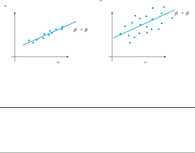
The parameter s

determines the amount of variability inherent in the regression

model. A large value of s

will lead to observed (x

, y

)’s that are quite spread out

about the true regression line, whereas whe n s

is small the observed points will

tend to fall very close to the true line (see Figure 12.11). An estimate of s

will be

used in confidence interval (CI) formulas and hypothesis-testing procedures pre-

sented in the next two sections. Because the equation of the true line is unknow n,

the estimate is based on the extent to which the sample observations deviate from

the estimated line. Many large deviations (residuals) suggest a large value of s

whereas if all deviations are small in magnitude it indicates that s

is small.

DEFINITION

The fitted (or predicted) values

;

; ...;

are obtained by successively

substituting the x values x

, ..., x

into the equation of the estimated regres-

sion line:

;

; ...;

. The residuals

are the vertical deviations y



; y



; ...; y



from the estimated

line.

In words, the predicted value

is the value of y that we would predict or expect

when using the estimated regression line with x ¼ x

;

is the height of the

estimated regression line above the value x

for which the ith observation was

made. The residual y



is the difference between the observed y

and the

predicted

. If the residuals are all small in mag nitude, then much of the variability

y Elongation

x Tensile force

y Product sales

Advertisin

expenditure

0 1

Figure 12.11 Typical sample for s

: (a) small; (b) large

12.2 Estimating Model Parameters 629

in observed y values appears to be due to the linear relationship between x and y,

whereas many large residuals suggest quite a bit of inherent variability in y relative

to the amount d ue to the linear relation. Assuming that the line in Figure 12.9 is the

least squares line, the residuals are identified by the vertical line segments from

the observed points to the line. When the estimated regress ion line is obtained

via the principle of least squares, the sum of the residuals should in theory be zero

(an immediate consequence of the first normal equation; see Exercise 24). In

practice, the sum may deviate a bit from zero due to rounding.

Example 12.7 Japan’s high population density has resulted in a multitude of resource usage

problems. One especially serious difficulty concerns waste removal. The article

“Innovative Sludge Handling Through Pelletization Thickening” (Water Res.,

1999: 3245–3252) reported the development of a new compression machine for

processing sewage sludge. An important part of the investigation involved relating

the moisture content of compressed pellets ( y, in %) to the machine’s filtration rate

(x, in kg-DS/m/h). The following data was read from a graph in the paper:

x 125.3 98.2 201.4 147.3 145.9 124.7 112.2 120.2 161.2 178.9

y 77.9 76.8 81.5 79.8 78.2 78.3 77.5 77.0 80.1 80.2

x 159.5 145.8 75.1 151.4 144.2 125.0 198.8 132.5 159.6 110.7

y 79.9 79.0 76.7 78.2 79.5 78.1 81.5 77.0 79.0 78.6

Relevant summary quantities (summary statistics) are

¼ 2817:9,

1574:8,

¼ 415;949:85,

¼ 222;657:88, and

¼ 124;039:58,

from which

x ¼ 140:895, y ¼ 78:74, S

¼ 18;921:8295, and S

¼ 776:434. Thus

776:434

18;921:8295

¼ :04103377  :041

¼78:74 ð:04103377Þð140:895Þ¼72:958547  72:96

from which the equation of the least squares line is

y ¼ 72:96 þ :041x. For numerical

accuracy, the fitted values are calculated from

¼ 72:958547 þ :04103377x

¼ 72:958547 þ :04103377 125:3ðÞ78:100 y



200; etc:

A positive residual corresponds to a point in the scatter plot that lies above the graph

of the least squares line, whereas a negative residual resu lts from a point lying

below the line. All predicted values (fits) and residuals appear in the accompanying

table.

Obs Filtrate Moistcon Fit Residual

1 125.3 77.9 78.100 0.200

2 98.2 76.8 76.988 0.188

3 201.4 81.5 81.223 0.277

4 147.3 79.8 79.003 0.797

5 145.9 78.2 78.945 0.745

6 124.7 78.3 78.075 0.225

7 112.2 77.5 77.563 0.063

8 120.2 77.0 77.891 0.891

630

CHAPTER 12 Regression and Correlation

9 161.2 80.1 79.573 0.527

10 178.9 80.2 80.299 0.099

11 159.5 79.9 79.503 0.397

12 145.8 79.0 78.941 0.059

13 75.1 76.7 76.040 0.660

14 151.4 78.2 79.171 0.971

15 144.2 79.5 78.876 0.624

16 125.0 78.1 78.088 0.012

17 198.8 81.5 81.116 0.384

18 132.5 77.0 78.396 1.396

19 159.6 79.0 79.508 0.508

20 110.7 78.6 77.501 1.099

■

In much the same way that the deviations from the mean in a one-sample

situation were combined to obtain the estimate s

ðx

 xÞ

=ðn  1Þ, the

estimate of s

in regression analysis is based on squaring and summing the

residuals. We will continue to use the symbol s

for this estimated variance, so

don’t confuse it with our previous s

DEFINITION

The error sum of squares (equivalently, residual sum of squares), denoted

by SSE, is

SSE ¼

ðy



½y

ð

Þ

and the least squares estimate of s

¼ s

SSE

n  2

ðy



n  2

The divisor n  2ins

is the number of degrees of freedom (df) associated with the

estimate (or, equivalently, with the error sum of squares). This is because to obtain

, the two parameters b

and b

must first be estimated, which results in a loss of

2 df (just as m had to be estimated in one-sample problems, resulting in an estimated

variance based on n  1 df). Replacing each y

in the formula for s

by the rv Y

gives the estimator S

. It can be shown that S

is an unbiased estimator for

(although the estimator S is biased for s). The mle of s

has divisor n rather

than n  2, so it is biased.

Example 12.8

(Example 12.7

continued)

The residuals for the filtration rate–moi sture content data were calculated previ-

ously. The corresponding error sum of squares is

SSE ¼ð:200Þ

þð:188Þ

þþð1:099Þ

¼ 7:968

The estimate of s

is then

¼ s

¼ 7:968=ð20  2Þ¼:4427, and the estimated

standard deviation is

s ¼ s ¼

ﬃﬃﬃﬃﬃﬃﬃﬃﬃﬃﬃ

:4427

¼ :665. Roughly speaking, .665 is the mag-

nitude of a typical deviation from the estimated regression line.

■

12.2 Estimating Model Parameters 631

Computation of SSE from the defini ng formula involves much tedious

arithmetic because both the predicted values and residuals must first be calculated.

Use of the following computational formula does not require these quantities.

SSE ¼



This expre ssion results from substituting y

into

ðy



, squaring

the summand, carrying the sum through to the resulting three terms, and simplify-

ing (see Exercise 24). This computational formula is especially sensitive to the

effects of rounding in

and

, so use as many digits as your calculator will

provide.

Example 12.9 The article “Promising Quantitative Nondestructive Evaluation Techniques for

Composite Materials” (Mater. Eval., 1985: 561–565) reports on a study to investi-

gate how the propagation of an ultrasonic stress wave through a substance depends

on the properties of the substance. The accompanying data on fracture strength

(x, as a percentage of ultimate tensile strength) and attenuation ( y, in neper/cm, the

decrease in amplitude of the stress wave) in fiberglass-reinforced polyest er com-

posites was read from a graph that appeared in the article. The simple linear

regression model is suggested by the substantial linear pattern in the scatter plot.

x 12 30 36 40 45 57 62 67 71 78 93 94 100 105

y 3.3 3.2 3.4 3.0 2.8 2.9 2.7 2.6 2.5 2.6 2.2 2.0 2.3 2.1

The necessary summary quantities are n ¼ 14,

¼ 890,

¼ 67;182,

¼ 37:6,

¼ 103:54,

¼ 2234:30, from which S

10;603:4285714, S

¼155:98571429,

¼:0147109, and

¼ 3:6209072.

The computational formula for SSE gives

SSE ¼ 103:54 ð3:6209072Þð37:6Þð:0147109Þð2234:30Þ¼:2624532

so s

¼ .2624532/12 ¼ .0218711 and s ¼ .1479. With rounding to three decimal

digits in the computational formula for SSE, the result is

SSE ¼ 104 ð3:62Þð37:6Þð:0147Þð2234:30Þ¼104  103:331 ¼ :669

which is wrong in all digits. The problem is that, even though each of the three

terms may be correct in its first three nonzero digits, the three correct digits can be

subtracted away, leaving you with no correct digits.

■

The Coefﬁcient of Determination

Figure 12.12 shows three different scatter plots of bivariate data. In all three plots,

the heights of the different points vary substantially, indicating that there is much

variability in observed y values. The points in the first plot all fall exactly on a

straight line. In this case, all (100% ) of the sample variation in y can be attributed to

632 CHAPTER 12 Regression and Correlation

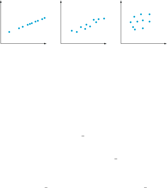
the fact that x and y are linearly related in combination with variation in x. The

points in Figure 12.12 b do not fall exactly on a line, but compared to overall y

variability, the deviations from the least squares line are small. It is reasonable to

conclude in this case that much of the observed y variation can be attributed to the

approximate linear relationship between the variables postulated by the simple

linear regression model. When the scatter plot looks lik e that of Figure 12.12c,

there is substantial variation about the least squares line relative to overall y

variation, so the simple linear regression model fails to explain variation in y by

relating y to x.

The error sum of squares SSE can be interpreted as a measure of how much

variation in y is left unexplained by the model—that is, how much cannot be

attributed to a linear relationship. In Figure 12.12a, SSE ¼ 0, and there is no

unexplained variation, whereas unexplai ned variation is small for the data of

Figure 12.12b and much larger in Figure 12.12c. A quantitative measur e of the

total amount of variation in observed y values is given by the total sum of squares

SST ¼ S

ðy

 yÞ

ð

The total sum of squares is the sum of squared deviations about the sample

mean of the observed y values. Thus the same number

y is subtracted from each y

SST, whereas SSE involves subtracting each different predicted value

from the

corresponding observed y

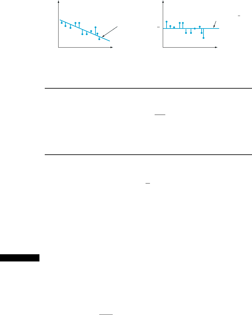
. Just as SSE is the sum of squared deviations about

the least squares line y ¼

x, SST is the sum of squared deviations about the

horizontal line at height

y (since then vertical deviations are y

 y), as pictured in

Figure 12.13. Furthermore, because the sum of squared deviations about the least

squares line is smaller than the sum of squared deviations about any other line,

SSE < SST unless the horizontal line is the least squares line. The ratio SSE/SST

is the proportion of total variation that cannot be explained by the simple linear

regression model, and 1  SSE/SST (a number between 0 and 1) is the proportion

of observed y variation explained by the model.

abc

Figure 12.12 Explaining y variation: (a) all variation explained; (b) most

variation explained; (c) little variation explained

12.2 Estimating Model Parameters 633

DEFINITION

The coefficient of determination, denot ed by r

, is given by

¼ 1 

SSE

SST

It is interpreted as the proportion of observed y variation that can be

explained by the simple linear regression model (attributed to an approximate

linear relationship between y and x).

In equivalent words, r

is the proportion by which the error sum of squares is

reduced by the regression line compared to the horizontal line. For example, if

SST ¼ 20 and SSE ¼ 2, then r

¼ 1 

, so the regression reduces the error sum

of squares by .90 ¼ 90%.

The higher the value of r

, the more successful is the simple linear regression

model in explaining y variation. When regression analysis is done by a statistical

computer package, either r

or 100r

(the percentage of variation explained by the

model) is a prominent part of the output. If r

is small, an analyst may want to

search for an alternative model (either a nonlinear model or a mul tiple regression

model that involves more than a single independent variable) that can more

effectively explain y variation.

Example 12.10

(Example 12.5

continued)

The scatter plot of the CO

concentration data in Figure 12.10 indicates a fairly high

value. With

¼2:349293

¼ :00845443 Sy

¼ 22:7

¼ 15; 441:4 Sy

¼ 78:93

we have

SST ¼78:93 

22:7

¼ 14:519

SSE ¼78:93 ð2:349293Þð22:7Þð:00845443Þð15;441 :4Þ¼1 :711

Least squares line

Horizontal line at height y

Figure 12.13 Sums of squares illustrated: (a) SSE ¼ sum of squared deviations about

the least squares line; (b) SST ¼ sum of squared deviations about the horizontal line

634

CHAPTER 12 Regression and Correlation

The coefficient of determination is then

¼ 1 

1:711

14:519

¼ 1  :118 ¼ :882

That is, 88.2% of the observed variation in mass is attributable to (can be explained

by) the approximate li near relationship between mass and CO

concentration, a

fairly impressive result. The r

can also be interpreted by saying that the error sum

of squares using the regression line is 88.2% less than the error sum of squares

using a horizontal line. By the way, although it is common to have r

values of .88

or more in engineering, the physical sciences, and the biological sciences, r

likely to be much smaller in social sciences such as psychology and sociology. An

as big as .5 would be unusual in predicting one test score from another. In

particular, when third grade verbal IQ score is used to predict third-grade written IQ

score for the 33 students of Example 1.2, r

is only .28.

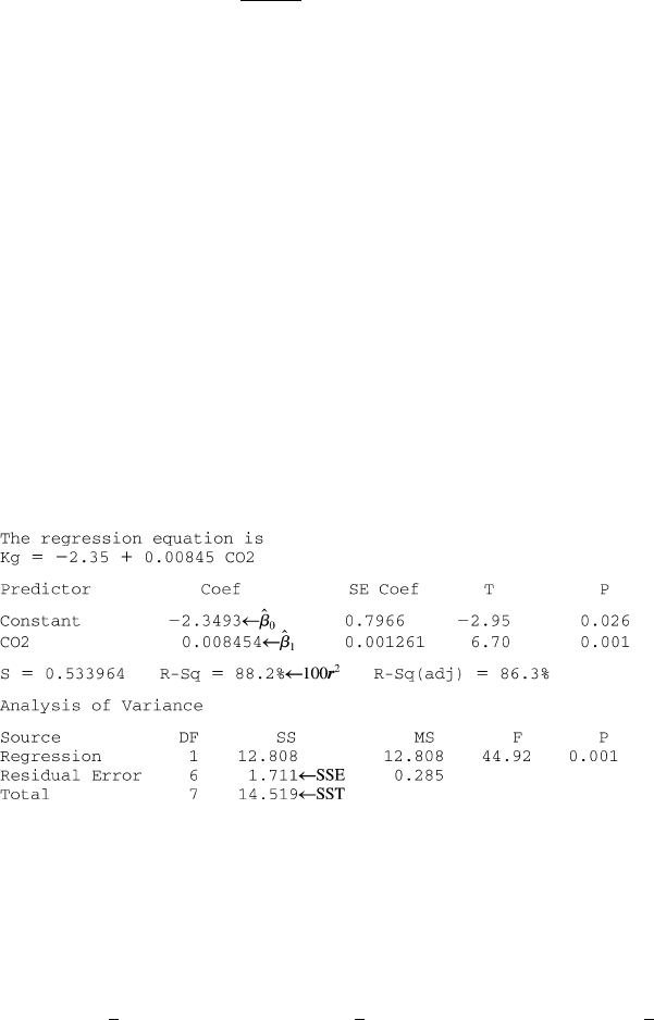
Figure 12.14 shows partial MINITAB output for the CO

concentration data

of Examples 12.5 and 12.10; the package will also provide the predicted values and

residuals upon request, as well as other information. The formats used by other

packages differ slightly from that of MINITAB, but the information content is very

similar. Quantities such as the standard deviations, t-ratios, and the details of the

ANOVA table are discussed in Section 12.3.

For regression there is an analysis of variance identity like the fundamental

identity (11.1), in Section 11.1. Add and subtract

in the total sum of squares:

SST ¼

ðy

 yÞ

½ðy



Þþð

 yÞ

ðy



 yÞ

Notice that the middle (cross-product) term is missing on the right, but see Exercise

24 for the justification. Of the two sums on the right, the first is SSE ¼

ðy



Figure 12.14 MINITAB output for the regression of Examples 12.5 and 12.10 ■

12.2 Estimating Model Parameters 635

and the second is something new, the regression sum of squares, SSR ¼

 yÞ

. Interpret the regression sum of squares as the amount of total variation

that is explained by the model. The analysis of varianc e identity for regression is

SST ¼ SSE þ SSR ð12:4Þ

The coefficient of determination in Example 12.10 can now be written in a

slightly different way:

¼ 1 

SSE

SST

SST  SSE

SST

SSR

SST

the ratio of explained variation to total variation. The ANOVA table in Figure 12.14

shows that SSR ¼ 12: 808, from which r

¼ 12:808=14:519 ¼ :882.

Terminology and Scope of Regression Analysis

The term regression analysis was first used by Francis Galton in the late nineteenth

century in connection with his work on the relationship between father’s height

x and son’s height y. After collecting a number of pairs (x

, y

), Galton used the

principle of least squares to obtain the equation of the estimated regression line

with the objective of using it to predict son’s height from father’s height. In using

the derived line, Galton found that if a father was above average in height, the son

would also be expected to be above average in height, but not by as much as the

father was. Similarly, the son of a shorter-than-aver age father would also be

expected to be shorter than average, but not by as much as the father. Thus the

predicted height of a son was “pulled back in” toward the mean; because regression

can be defined as moving backward, Galton adopted the terminology regression

line. This phenomenon of being pulled back in toward the mean has been observed

in many other situations (e.g., batting averages from year to year in b aseball) and is

called the regression effect or regression to the mean. See also Section 5.3 for a

discussion of this topic in the context of the bivariate normal distribution.

Because of the regression effect, care must be exer cised in experiments that

involve selecting individuals based on below average scores. For example, if

students are selected because of below average performance on a test, and they

are then given special instruction, then the regression effect predicts improvement

even if the instruction is useless. A similar warning applies in studies of under-

performing businesses or hospital patients.

Our discussion thus far has presumed that the independent variable is under

the control of the investigator, so that only the dependent variable Y is random. This

was not, however, the case with Galton’s experiment; fathers’ heights were not

preselected, but instead both X and Y were random. Methods and conclusions of

regression analysis can be applied both when the valu es of the independent variable

are fixed in advance and when they are random, but because the derivations and

interpretations are more straightforward in the former case, we will continue to

work explicitly with it. For more comme ntary, see the excellent book by Michael

Kutner et al. listed in the chapter bibliography.

636 CHAPTER 12 Regression and Correlation

Exercises Section 12.2 (13–30)

13. Exercise 4 gave data on x ¼ BOD mass loading

and y ¼ BOD mass removal. Values of relevant

summary quantities are

n ¼ 14

¼ 517

¼ 346

¼ 39;095

¼ 17;454

¼ 25;825

a. Obtain the equation of the least squares line.

b. Predict the value of BOD mass removal for a

single observation made when BOD mass

loading is 35, and calculate the value of the

corresponding residual.

c. Calculate SSE and then a point estimate of s.

d. What proportion of observed variation in

removal can be explained by the approximate

linear relationship between the two variables?

e. The last two x values, 103 and 142, are much

larger than the others. How are the equation of

the least squares line and the value of r

affected by deletion of the two corresponding

observations from the sample? Adjust the

given values of the summary quantities, and

use the fact that the new value of SSE is

311.79.

14. The accompanying data on x ¼ current density

(mA/cm

) and y ¼ rate of deposition (mm/min)

appeared in the article “Plating of 60/40 Tin/

Lead Solder for Head Termination Metallurgy”

(Plating and Surface Finishing, Jan. 1997:

38–40). Do you agree with the claim by the

article’s author that “a linear relationship was

obtained from the tin–lead rate of deposition as

a function of current density”? Explain your

reasoning.

x 20 40 60 80

y .24 1.20 1.71 2.22

15. Refer to the data given in Exercise 1 on tank

temperature and efficiency ratio.

a. Determine the equation of the estimated

regression line.

b. Calculate a point estimate for true average

efficiency ratio when tank temperature is 182.

c. Calculate the values of the residuals from the

least squares line for the four observations for

which temperature is 182. Why do they not all

have the same sign?

d. What proportion of the observed variation in

efficiency ratio can be attributed to the simple

linear regression relationship between the two

variables?

16. As an alternative to the use of father’s height to

predict son’s height, Galton also used the mid-

parent height, the average of the father’s and

mother’s heights. Here are the heights of 11

female students along with their midparent

heights in inches:

Midparent 66.0 65.5 71.5 68.0 70.0 65.5 67.0

Daughter 64.0 63.0 69.0 69.0 69.0 65.0 63.0

Midparent 70.5 69.5 64.5 67.5

Daughter 68.5 69.0 64.0 67.0

a. Make a scatter plot of daughter’s height

against the midparent height and comment

on the strength of the relationship.

b. Is the daughter’s height completely and

uniquely determined by the midparent

height? Explain.

c. Use the accompanying MINITAB output to

obtain the equation of the least squares line

for predicting daughter height from midparent

height, and then predict the height of a daugh-

ter whose midparent height is 70 in. Would

you feel comfortable using the least squares

line to predict daughter height when midpar-

ent height is 74 in.? Explain.

Predictor Coef SE Coef T P

Constant 1.65 13.36 0.12 0.904

midparent 0.9555 0.1971 4.85 0.001

S ¼ 1.45061 R-Sq ¼ 72.3% R-Sq(adj) ¼69.2%

Analysis of Variance

Source DF SS MS F P

Regression 1 49.471 49.471 23.51 0.001

Residual 9 18.938 2.104

Error

Total 10 68.409

d. What are the values of SSE, SST, and the

coefficient of determination? How well does

the midparent height account for the variation

in daughter height?

e. Notice that for most of the families, the mid-

parent height exceeds the daughter height. Is

this what is meant by regression to the mean?

Explain.

17. The article “Characterization of Highway Runoff

in Austin, Texas, Area” (J. Environ. Engrg.,

1998: 131–137) gave a scatter plot, along with

12.2 Estimating Model Parameters 637