Devore J.L., Berk K.N. Modern Mathematical Statistics with Applications

Подождите немного. Документ загружается.

the least squares line, of x ¼ rainfall volume

) and y ¼ runoff volume (m

) for a particular

location. The accompanying values were read

from the plot.

x 5 12141723304047

y 4 10131515252746

x 55 67 72 81 96 112 127

y 38 46 53 70 82 99 100

a. Does a scatter plot of the data support the use

of the simple linear regression model?

b. Calculate point estimates of the slope and

intercept of the population regression line.

c. Calculate a point estimate of the true average

runoff volume when rainfall volume is 50.

d. Calculate a point estimate of the standard

deviation s.

e. What proportion of the observed variation in

runoff volume can be attributed to the simple

linear regression relationship between runoff

and rainfall?

18. A regression of y ¼ calcium content (g/L) on

x ¼ dissolved material (mg/cm

) was reported

in the article “Use of Fly Ash or Silica Fume to

Increase the Resistance of Concrete to Feed

Acids” (Mag. Concrete Res., 1997: 337–344).

The equation of the estimated regression line

was y ¼ 3.678 + .144x, with r

¼ .860, based

on n ¼ 23.

a. Interpret the estimated slope .144 and the

coefficient of determination .860.

b. Calculate a point estimate of the true average

calcium content when the amount of dis-

solved material is 50 mg/cm

c. The value of total sum of squares was SST

¼ 320.398. Calculate an estimate of the error

standard deviation s in the simple linear

regression model.

19. The cetane number is a critical property in spe-

cifying the ignition quality of a fuel used in a

diesel engine. Determination of this number for a

biodiesel fuel is expensive and time-consuming.

The article “Relating the Cetane Number of Bio-

diesel Fuels to Their Fatty Acid Composition:

A Critical Study” (J. Automobile Engr., 2009:

565–583) included the following data on x ¼

iodine value (g) and y ¼ cetane number for a

sample of 14 biofuels. The iodine value is the

amount of iodine necessary to saturate a sample

of 100 g of oil. The article’s authors fit the simple

linear regression model to this data, so let’s fol-

low their lead.

x 132.0 129.0 120.0 113.2 105.0 92.0 84.0

y 46.0 48.0 51.0 52.1 54.0 52.0 59.0

x 83.2 88.4 59.0 80.0 81.5 71.0 69.2

y 58.7 61.6 64.0 61.4 54.6 58.8 58.0

¼1307:5;

¼779:2;

¼128;913:93;

¼71;347:30;

¼43;745:22

a. Obtain the equation of the least squares line,

and then calculate a point prediction of the

cetane number that would result from a single

observation with an iodine value of 100.

b. Calculate and interpret the coefficient of

determination.

c. Calculate and interpret a point estimate of the

model standard deviation s.

20. A number of studies have shown lichens (certain

plants composed of an alga and a fungus) to be

excellent bioindicators of air pollution. The arti-

cle “The Epiphytic Lichen Hypogymnia phy-

sodes as a Biomonitor of Atmospheric Nitrogen

and Sulphur Deposition in Norway” (Environ.

Monitoring Assessment, 1993: 27–47) gives the

following data (read from a graph) on x ¼ NO



wet deposition (g N/m

) and y ¼ lichen N (% dry

weight):

x .05 .10 .11 .12 .31 .37 .42

y .48 .55 .48 .50 .58 .52 1.02

x .58 .68 .68 .73 .85 .92

y .86 .86 1.00 .88 1.04 1.70

The author used simple linear regression to ana-

lyze the data. Use the accompanying MINITAB

output to answer the following questions:

a. What are the least squares estimates of b

and

b. Predict lichen N for an NO



deposition

value of .5.

c. What is the estimate of s?

d. What is the value of total variation, and how

much of it can be explained by the model

relationship?

638

CHAPTER 12 Regression and Correlation

The regression equation is lichen

N ¼ 0.365

+ 0.967 no3 depo

Predictor Coef Stdev t-ratio P

Constant 0.36510 0.09904 3.69 0.004

no3 depo 0.9668 0.1829 5.29 0.000

S ¼ 0.1932 R-sq ¼ 71.7% R-sq (adj) ¼ 69.2%

Analysis of Variance

Source DF SS MS F P

Regression 1 1.0427 1.0427 27.94 0.000

Error 11 0.4106 0.0373

Total 12 1.4533

21. The article “Effects of Bike Lanes on Driver and

Bicyclist Behavior” (ASCE Transportation

Engrg. J., 1977: 243–256) reports the results of

a regression analysis with x ¼ available travel

space in feet (a convenient measure of roadway

width, defined as the distance between a cyclist

and the roadway center line) and separation dis-

tance y between a bike and a passing car (deter-

mined by photography). The data, for ten streets

with bike lanes, follows:

x 12.8 12.9 12.9 13.6 14.5

y 5.5 6.2 6.3 7.0 7.8

x 14.6 15.1 17.5 19.5 20.8

y 8.3 7.1 10.0 10.8 11.0

a. Verify that

¼ 154:20,

¼ 80,

¼ 2452:18,

¼ 1282:74, and

¼ 675:16.

b. Derive the equation of the estimated regres-

sion line.

c. What separation distance would you predict

for another street that has 15.0 as its available

travel space value?

d. What would be the estimate of expected sep-

aration distance for all streets having avail-

able travel space value 15.0?

22. For the past decade rubber powder has been used

in asphalt cement to improve performance. The

article “Experimental Study of Recycled Rubber-

Filled High-Strength Concrete” (Mag. Concrete

Res., 2009: 549–556) included on a regression of

y ¼ axial strength (MPa) on x ¼ cube strength

(MPa) based on the following sample data:

x 112.3 97.0 92.7 86.0 102.0

y 75.0 71.0 57.7 48.7 74.3

x 99.2 95.8 103.5 89.0 86.7

y 73.3 68.0 59.3 57.8 48.5

a. Verify that a scatter plot supports the assump-

tion that the two variables are related via the

simple linear regression model.

b. Obtain the equation of the least squares line,

and interpret its slope.

c. Calculate and interpret the coefficient of deter-

mination

d. Calculate and interpret an estimate of the error

standard deviation s in the simple linear

regression model.

e. The largest x value in the sample considerably

exceeds the other x values. What is the effect

on the equation of the least squares line of

deleting the corresponding observation?

23. Show that the mle’s of b

and b

are indeed the

least squares estimates. [Hint: The pdf of Y

normal with mean m

¼ b

+ b

and variance

; the likelihood is the product of the n pdf’s.]

24. Denote the residuals by e

; ...; e

ðe

¼ y



a. Show that

¼ 0 and

¼ 0. [Hint:

Examine the two normal equations.]

b. Show that

 y ¼

ðx

 xÞ.

c. Use (a) and (b) to derive the analysis of vari-

ance identity for regression, Equation (12.4),

by showing that the cross-product term is 0.

d. Use (b) and Equation (12.4) to verify the

computational formula for SSE.

25. A regression analysis is carried out with y ¼ tem-

perature, expressed in



C. How do the resulting

values of

and

relate to those obtained if y is

reexpressed in



F? Justify your assertion. [Hint:

new y

¼ y

¼ 1:8y

þ 32:]

26. Show that b

and b

of Expressions ( 12.2 ) and

(12.3) satisfy the normal equations.

27. Show that the “point of averages” ð

x; yÞ lies on the

estimated regression line.

28. Suppose an investigator has data on the amount

of shelf space x devoted to display of a particular

product and sales revenue y for that product. The

investigator may wish to fit a model for which

the true regression line passes through (0, 0).

The appropriate model is Y ¼ b

x+e. Assume

that (x

, y

), ...,(x

, y

) are observed pairs gener-

ated from this model, and derive the least squares

estimator of b

.[Hint: Write the sum of squared

deviations as a function of b

, a trial value, and use

calculus to find the minimizing value of b

12.2 Estimating Model Parameters 639

29. a. Consider the data in Exercise 20. Suppose that

instead of the least squares line passing through

the points (x

, y

), ...,(x

, y

), we wish the

least squares line passing through

ðx

 x; y

Þ; ...; ðx

 x; y

Þ. Construct a

scatter plot of the (x

, y

) points and then of

the ðx

 x; y

Þ points. Use the plots to explain

intuitively how the two least squares lines are

related to each other.

b. Suppose that instead of the model

¼ b

þ b

þ e

i ¼ 1; ...; nðÞ, we wish

to fit a model of the form

¼ b



þ b



ðx

 xÞþe

i ¼ 1; ...; nðÞ.

What are the least squares estimators of b



and



, and how do they relate to

and

30. Consider the following three data sets, in which

the variables of interest are x ¼ commuting dis-

tance and y ¼ commuting time. Based on a scatter

plot and the values of s and r

, in which situation

would simple linear regression be most (least)

effective, and why?

12 3

xyx y x y

15 42 5 16 5 8

16 35 10 32 10 16

17 45 15 44 15 22

18 42 20 45 20 23

19 49 25 63 25 31

20 46 50 115 50 60

17.50 1270.8333 1270.8333

29.50 2722.5 1431.6667

1.685714 2.142295 1.126557

13.666672 7.868852 3.196729

SST 114.83 5897.5 1627.33

SSE 65.10 65.10 14.48

12.3

Inferences About the Regression

Coefficient



In virtually all of our inferential work thus far, the notion of sampling variability

has been pervasive. In particular, properties of sampling distributions of various

statistics have been the basis for developing confidence interval formulas and

hypothesis-testing methods. The key idea here is that the value of virtually any

quantity calculated from sample data—the value of virtually any statistic—is going

to vary from one sample to another.

Example 12.11 Re consider the global warming data on x ¼ CO

and y ¼ tree growth mass from

Example 12.5 in the previous section. There are 8 observations, 2 at each of the x

values 408, 554, 680, and 812. Suppose that the slope and intercept of the true

regression line are b

¼ .0085 and b

¼2.35, with s ¼ .5 (consistent with the

values

¼ :00845,

¼2:349, s ¼ 0:534, computed in Example 12.10). Using

R, we proceeded to generate a sample of random deviations

; ...;

from a

normal distribution with mean 0 and standard deviation .5, and then added

+ b

to obtain 8 corresponding y values. Regression calculations were then

carried out to obtain the estimated slope, intercept, and standard deviation. This

process was repeated a total of 20 times, resulting in the values given in Table 12.1 .

There is clearly variat ion in values of the estimated slope and estimated

intercept, as well as the estimated standar d deviation. The equation of the least

squares line thus varies from one sample to the n ext. Figure 12.15 shows graphs of

the true regression line and the 20 sample regression lines.

640 CHAPTER 12 Regression and Correlation

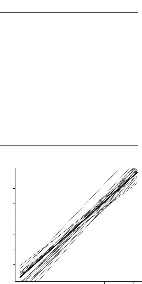
Table 12.1 Sim ulation results for Example 12.11

1 2.606 0.0086 0.312

2 3.639 0.0104 0.345

3 3.316 0.0100 0.530

4 3.042 0.0093 0.475

5 3.400 0.0103 0.441

6 3.932 0.0107 0.328

7 2.533 0.0090 0.423

8 2.862 0.0100 0.676

9 2.152 0.0081 0.401

10 2.975 0.0093 0.409

11 2.255 0.0084 0.639

12 3.003 0.0095 0.437

13 3.187 0.0093 0.587

14 2.424 0.0087 0.598

15 1.490 0.0073 0.735

16 1.812 0.0074 0.332

17 1.845 0.0079 0.552

18 4.080 0.0107 0.520

19 2.958 0.0090 0.718

20 1.670 0.0072 0.574

400 500 600 700 800

CO2

4.5

4.0

3.5

3.0

2.5

2.0

1.5

1.0

mass

Figure 12.15 Simulation results from Example 12.11: graphs of the true

regression line and 20 least squares lines (from R) ■

12.3 Inferences About the Regression Coefﬁcient b

641

The slope b

of the population regression line is the true average change in the

dependent variable y associated with a 1-unit increase in the independent variable x.

The slope of the least squares line,

, gives a point estimate of b

. In the same way

that a confidence interval for m and procedures for testing hypotheses about m were

based on properties of the sampling distribution of

X, further inferences about b

are

based on thinking of

as a statistic and investigating its sampling distribution.

The values of the x

’s are assumed to be chosen before the experiment is

performed, so only the Y

’s are random. The estimators (statistics, and thus random

variables) for b

and b

are obtained by replacing y

by Y

in (12.2) and (12.3):

ðx

 xÞðY

 YÞ

ðx

 xÞ

;



Similarly, the estimator for s

results from replacing each y

in the formula for s

the rv Y

¼ S



n  2

The denominator of

, S

ðx

 xÞ

, depends only on the x

’s and not

on the Y

’s, so it is a constant. Then because

ðx

 xÞY ¼ Y

ðx

 xÞ¼

Y  0 ¼ 0, the slope estimator can be written as

ðx

 xÞY

where c

¼ðx

 xÞ=S

That is,

is a linear function of the independent rv’s Y

, Y

, ..., Y

, each of which

is normally distributed. Invoking properties of a linear funct ion of random variables

discussed in Section 6.3 leads to the following results (Exercise 40).

1. Th e mean value of

is Eð

Þ¼m

¼ b

,so

is an unbiased estimator

of b

(the distribution of

is always centered at the value of b

2. Th e variance and standard deviation of

are

Vð

Þ¼s

ﬃﬃﬃﬃﬃﬃ

ð12:5Þ

where S

ðx

 xÞ



ðÞ

=n. Replacing s by its estimate

s gives an estimate for s

(the estimated standard deviation, i.e., estimated

standard error, of

ﬃﬃﬃﬃﬃﬃ

(This estimate can also be denoted by

3. Th e estimator

has a normal distribution (because it is a linear function

of independent normal rv’s).

642 CHAPTER 12 Regression and Correlation

According to (12.5), the variance of

equals the variance s

of the random error

term—or, equivalently, of any Y

—divided by

ðx

 xÞ

. Because

ðx

 xÞ

a measure of how spread out the x

’s are about x, we conclude that making

observations at x

values that are quite spread out results in a more precise estimator

of the slope parameter (smaller variance of

), whereas values of x

all close to each

other imply a highly variable estimator. Of course, if the x

’s are spread out too far,

a linear model may not be appropriate throughout the range of observation.

Many inferential procedures discussed previously were based on standardiz-

ing an estimator by first subtracting its mean value and then dividing by its

estimated standard deviation. In particular, test procedures and a CI for the mean

m of a normal population utilized the fact that the standar dized variable

X  mÞ=ðS=

ﬃﬃﬃﬃﬃ

nÞ

—that is, ðX  mÞ=S

—had a t distribution with n 1 df. A similar

result here provides the key to further inferences concerni ng b

THEOREM

The assumptions of the simple linear regression model imply that the

standardized variable

T ¼

 b

ﬃﬃﬃﬃﬃﬃ

 b

has a t distribution with n  2 df.

The T ratio can be written as

T ¼

 b

ﬃﬃﬃﬃﬃﬃ

 b

ﬃﬃﬃﬃﬃﬃ

ﬃﬃﬃﬃﬃﬃﬃﬃﬃﬃﬃﬃﬃﬃﬃﬃﬃﬃﬃﬃﬃﬃﬃﬃﬃﬃ

ðn  2ÞS



ðn  2Þ

The theorem is a consequence of the following facts: ð

 b

Þ=ðs=

ﬃﬃﬃﬃﬃﬃ

Þ

N 0; 1ðÞ, ðn  2ÞS



 w

n2

, and

is independent of S

. That is, T is a standard

normal rv divided by the square root of an independent chi-squared rv over its df, so

T has the specified t distribution.

A Conﬁdence Interval for b

As in the derivation of previous CIs, we begin with a probability statement:

P t

a=2;n2

 b

< t

a=2;n2

¼ 1  a

Manipulation of the inequalitie s inside the parentheses to isolate b

and substitution

of estimates in place of the estimators gives the CI formula.

12.3 Inferences About the Regression Coefﬁcient b

643

A 100(1  a)% CI for the slope b

of the true regression line is

 t

a=2;n2

 s

This interval has the same general form as did many of our previous intervals. It is

centered at the point estimate of the parameter, and the amount it extends out to

each side of the estimate depends on the desired confidence level (through the

t critical value) and on the amount of variability in the estimator

(through s

which will tend to be small when there is little variability in the distribution of

and large otherwise).

Example 12.12 Is it possible to predict graduation rates from freshman test scores? Based on

the average SAT score of entering freshmen at a university, can we predict the

percentage of those freshmen who will get a degree there within 6 years? We use a

random sample of 20 universities from the 248 national universities listed in the

2005 edition of America’s Best Colleges, published by U. S .News & World Report.

Rank University Grad rate SAT Private or State

1 2 Princeton 98 1465.00 P

2 13 Brown 96 1395.00 P

3 15 Johns Hopkins 88 1380.00 P

4 69 Pittsburgh 65 1215.00 S

5 77 SUNY-Binghamton 80 1235.00 S

6 94 Kansas 58 1011.10 S

7 102 Dayton 76 1055.54 P

8 107 Illinois Inst Tech 67 1166.65 P

9 125 Arkansas 48 1055.54 S

10 139 Florida Inst Tech 54 1155.00 P

11 147 New Mexico Inst Mining 42 1099.99 S

12 158 Temple 54 1080.00 S

13 172 Montana 45 944.43 S

14 174 New Mexico 42 899.99 S

15 178 South Dakota 51 944.43 S

16 183 Virginia Commonwealth 42 1060.00 S

17 186 Widener 70 1005.00 P

18 187 Alabama A&M 38 722.21 S

19 243 Toledo 44 877.77 S

20 245 Wayne State 31 833.32 S

The SAT scores were actually given in the form of first and third quarti les, so the

average of those two numbers is used here. Notice that some of the SAT scores are

not integers. Those values were computed from ACT scores using the NCAA

formula SAT ¼55.556 + 44.444ACT, which is equivalent to saying that there

is a linear relationship with 17 on the ACT corresponding to 700 on the SAT, and

26 on the ACT corresponding to 1100 on the SAT.

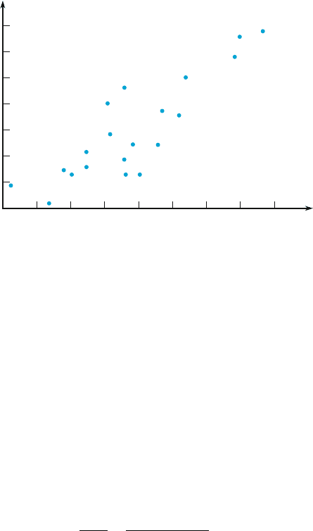
The scatter plot of the data in Figure 12.16 suggests the appropriateness of the

linear regression model; graduation rate increases approximately linearly with SAT.

644 CHAPTER 12 Regression and Correlation

The values of the summary statistics required for calculation of the least squares

estimates are

¼21;600:97

¼1189

¼24;034;220:545

¼1;346;524:53

¼78;113

from which S

¼ 62,346.86, S

¼ 704,125.298,

¼ :08854513,

36:1830309, SST ¼ 7426:95, SSE ¼ 1906:439, r

¼ 1  1906:439=7426: 95 ¼

:7433. Roughly 74% of the observed variation in graduation rate can be attributed to

the simple linear regression model relationship between graduation rate and SAT.

Error df is 20  2 ¼ 18, giving s

¼ 1906.439/18 ¼ 105.9 and s ¼ 10.29.

The estimated standard deviation of

ﬃﬃﬃﬃﬃﬃ

10:29

ﬃﬃﬃﬃﬃﬃﬃﬃﬃﬃﬃﬃﬃﬃﬃﬃﬃﬃﬃﬃﬃﬃﬃﬃﬃ

704;125:298

¼ :01226

The t critical value for a confidence level of 95% is t

.025,18

¼ 2.101. The confidence

interval is

:0885  2:101ðÞ:01226ðÞ¼:0885  :0258 ¼ :063 ;:114ðÞ

With a high degree of confidence, we estimate that an average increase in

percentage graduation rate of between .063 and .114 is associated with a 1 point

increase in SAT. Multiplying by 100 gives the change in graduation percentage

corresponding to a 100 point increase in SAT, 8.85  2.58, between 6.3 and 11.4.

This shows that a substantial increase in graduation rate accompanies an increase of

100 SAT points. Is this a causal relationship, so a university president can count on

an increased graduation rate if the admissions process becomes more selective in

terms of entrance exam scores? One can imagine contrary scenarios, such as that

more serious students attend more prestigious colleges, with higher entrance

requirements and higher graduation rates, and that prestige would not be affected

by an increase in entrance requirements. However, it seems more likely that

100

700 800 900 1000 1100 1200 1300 1400 1500

Grad. rate

SAT

Figure 12.16 Scatter plot of the data from Example 12.12

12.3 Inferences About the Regression Coefﬁcient b

645

prestige would benefit from higher test scores, so this scenario is not a very good

argument against causality. In any case, there is at least one university president

who claimed that increasing test scores resulted in a higher graduation rate.

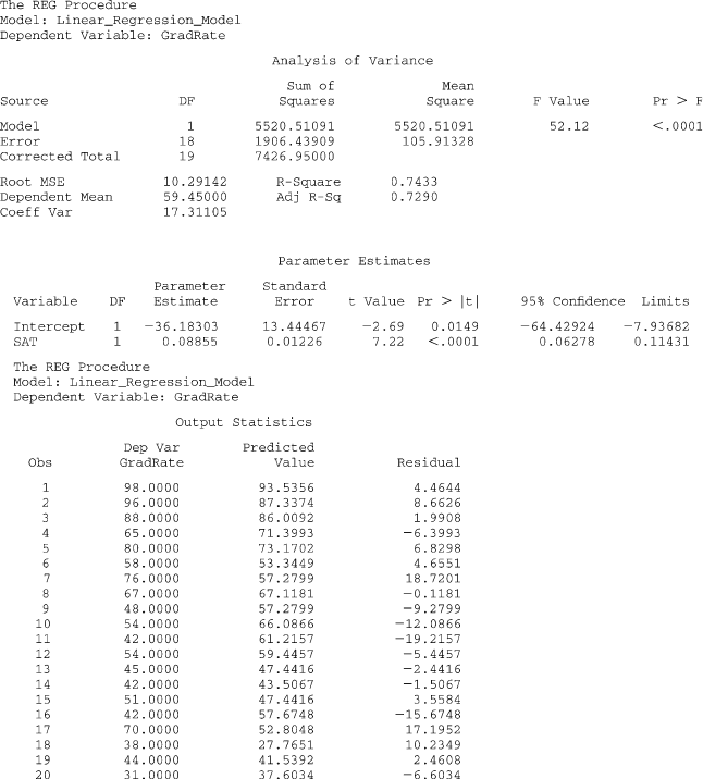
Looking at the SAS output of Figure 12.17, we find the value of s

under

Parameter Estimates as the second number in the Standard Error column. All of the

widely used statistical packages include this estimated standard error in output.

There is also an estimated standard error for the statistic

. Confidence intervals for

and b

appear on the output. For all of the statistics, compare the values on the

SAS output with the values that we calculated.

The output shows the values of graduation rate, predicted values, and residuals.

Matching the rows in Figure 12.17 with the corresponding rows in the original listing

of the data, it is possible to see that the residuals for the private universities are mostly

positive. However, it is much easier to see this in Figure 12.18,wheretheprivate

Figure 12.17 SAS output for the data of Example 12.12

646

CHAPTER 12 Regression and Correlation

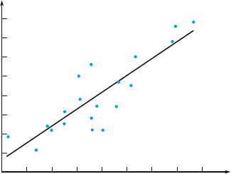
universities are labeled “P” and the public universities are labeled “S.” Of the seven

private universities, five are above their predictions (positive residual) and one is

barely below. Private universities mostly seem to achieve a higher graduation rate for

a given entrance exam score (for more on this issue, see the rest of the story in

Sections 12.6 and 12.7). It is interesting to speculate about why this might occur.

Is there a more nurturing atmosphere with more individual attention at private

schools? On the other hand, private universities might attract students who are

more likely to graduate regardless of the campus atmosphere.

■

Hypothesis-Testing Procedures

As before, the null hypothesis in a test about b

will be an equality statement. The

null value (value of b

claimed true by the null hypothesis) will be denoted by b

(read “beta one nought,” not “beta ten”). The test statistic results from replacing b

in the standardized variable T by the null value b

—that is, from standardizing the

estimator of b

under the assumption that H

is true. The test statistic thus has a

t distribution with n  2 df when H

is true, so the type I error probability is

controlled at the desired level a by using an appropriate t critica l value.

The most commonly encountered pair of hypotheses about b

is H

: b

¼ 0

versus H

: b

6¼ 0. When this null hypothesis is true, m

Yx

¼ b

independent of x,

so know ledge o f x gives no information about the value of the dependent variable.

A tes t of these two hypotheses is often referred to as the model utility test in simple

linear regression. Unless n is quite small, H

will be rejected and the utility of

the model confirmed precisely when r

is reasonably large. The simple linear

regression model should not be used for further inferences (estimates of mean

value or predictions of future values) unless the model utility test results in

rejection of H

for a suitably small a.

100

Grad. rate

700 800 900 1000 1100 1200 1300 1400 1500

SAT

Figure 12.18 Comparing private and state universities

12.3 Inferences About the Regression Coefﬁcient b

647