Devore J.L., Berk K.N. Modern Mathematical Statistics with Applications

Подождите немного. Документ загружается.

Null hypothesis: H

: b

¼ b

Test statistic value: t ¼

 b

Alternative Hypothesis Rejection Region for Level a Test

: b

> b

t  t

a,n2

: b

< b

t t

a,n2

: b

6¼ b

either t  t

a/2,n2

or t t

a/2,n2

A P-value based on n  2 df can be calculated just as was done previously for

t tests in Chapters 9 and 10.

The model utility test is the test of H

: b

¼ 0 versus H

: b

6¼ 0, in

which case the test statistic value is the t ratio t ¼

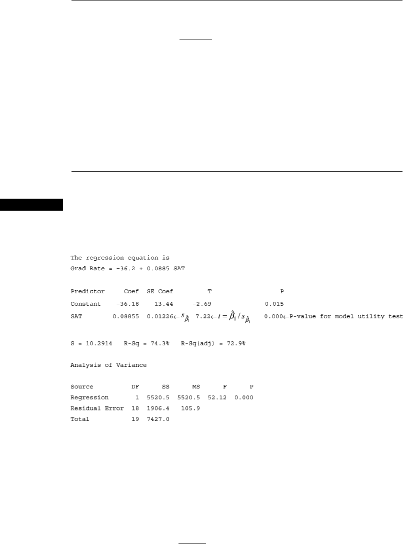
Example 12.13 Let’s carry out the model utility test at significance level a ¼ .05 for the data of

Example 12.12. We use the MINITAB regression ou tput in Figure 12.19, which can

be compared with the SAS output of Figure 12.17.

The parameter of interest is b

, the expected change in graduation rate

associated with an increase of 1 in SAT score. The null hypothesis H

: b

¼ 0

will be rejected in favor of the alternative H

: b

6¼ 0 if the t ratio t ¼

satisfies

either t  t

a/2,n2

¼ t

.025,18

¼ 2.101 or t 2.101.

From Figure 12.19,

¼ :08855, s

¼ :01226, and

t ¼

:08855

:01226

¼ 7:22 (also on output)

Figure 12.19 MINITAB output for Example 12.13

648

CHAPTER 12 Regression and Correlation

Clearly, 7.22  2.101, so H

is resoundingly rejected. Alternatively, the P-value is

twice the area captured under the 18 df t curve to the right of 7.22. MINITAB gives

P-value ¼ .000, so H

should be rejected at any reasonable a. This confirmation of

the utility of the simple linear regression model gives us license to calculate various

estimates and predictions as described in Section 12.4.

Notice that, in contrast, SAS in Figure 12.17 gives a P-value of < .0001.

This is better than the MINITAB P-value of .000 because the MINITAB value

could be incorrectly read as 0. Of course the actual value is positive, approximately

.0000010. When rounded to three decimals this gives the value .000 printed

by MINITAB.

Given the confidence interval of Example 12.12, the result of the hypothesis test

should be no surprise. It should be clear, in the two-tailed test for H

: b

¼ 0atlevela,

that H

is rejected if and only if the 100(1 a)% confidence interval fails to include 0.

In the present instance, the 95% confidence interval did not include 0, so we should

have known that the two-tailed test at level .05 would reject H

: b

¼ 0. ■

Regression and ANOVA

The splitting of the total sum of squares

ðy

 yÞ

into a part SSE, which

measures unexplained variation, and a part SSR, which measures variation

explained by the linear relationship, is strongly reminisc ent of one-way ANOVA.

In fact, the n ull hypothesis H

: b

¼ 0 can be tested against H

: b

6¼ 0by

constructing an ANOVA table (Table 12.2) and rejecting H

if f  F

a,1,n2

The F test gives exactly the same result as the model utility t test because

¼ f and t

a=2;n2

¼ F

;1;n2

. Virtually all computer packages that have regression

options include such an ANOVA table in the output. For example, Figur e 12.17

shows SAS output for the university data of Example 12.12. The ANOVA table at

the top of the output has f ¼ 52.12 with a P-value of <.0001 (the actual value is

about .0000010) for the model utility test. The table of parameter estimates gives

t ¼ 7.22, again with P ¼ <.0001 (the actual value is about .0000010) and t

¼ (7.22)

¼ 52.12 ¼ f.

Table 12.2 ANOVA table for simple linear regression

Source of variation df Sum of Squares Mean Square f

Regression 1 SSR SSR

SSR

SSE=ðn  2Þ

Error n  2 SSE

SSE

n  2

Total n  1 SST

12.3 Inferences About the Regression Coefﬁcient b

649

Fitting the Logistic Regression Model

Recall from Section 12.1 that in the logistic regression model, the dependent

variable Y is 1 if the observation is a success and 0 otherwise. The probability of

success is related to a quantitative predictor x by the logit function pðxÞ¼

þb

=ð1 þ e

þb

Þ. Fitting the model to sample data requires that the parameters

and b

be estimated. The standard way of doing this is by the method of

maximum likelihood. Suppose, for example, that n ¼ 5 and that the observations

made at x

, x

, and x

are successes whereas the other two observations are failures.

Then the likelihood function is

1  px

ðÞ½px

ðÞ½1  px

ðÞ½px

ðÞ½

1 þ e

þb



þb

1 þ e

þb



1 þ e

þb



þb

1 þ e

þb



þb

1 þ e

þb



Unfortunately it is not at all straightforward to maximize this likelihood, and there

are no nice formulas for the mle’s

and

The maximization process must be

carried out using iterative numerical methods. The details are involved, but fortu-

nately the most popular statistical software packages will do this on request and

provide quantitative and graphical indicati ons of how well the model fits.

In particular, the mle

is provided along with its estimated standard devia-

tion s

. For large n, the estimator has approximately a normal distribution and the

standardized variable ð

 b

Þ=S

has approximately a standard normal distribu-

tion. This allows for calculation of a confidence interval for b

as well as for testing

: b

¼ 0, according to which the value of x has no impact on the likelihood of

success. Some software packages report the value of the chi-squared statistic z

rather than z itself, along with the corresponding P-value for a two-tailed test.

Example 12.14 Here is data on launch temperature and the incidence of failure for O-rings in 23

space shuttle launches prior to the Challenger disaster of January 1986.

Temperature Failure Temperature Failure Temperature Failure

53 Y 68 N 75 N

57 Y 69 N 75 Y

58 Y 70 N 76 N

63 Y 70 N 76 N

66 N 70 Y 78 N

67 N 70 Y 79 N

67 N 72 N 81 N

67 N 73 N

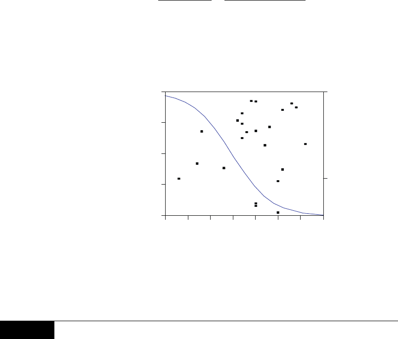
Figure 12.20 shows JMP output for a logistic regression analysis. We have chosen

to let p denote the probability of failure. Failures tended to occur at lower tem-

peratures and successes at higher temperatures, so the graph of

p decreases as

temperature increases. The estimate of b

¼:2322, and the estimated

standard deviation of

is s

¼ :1082. The value of z for testing H

: b

¼ 0,

which asserts that temperature does not affect the likelihood of O-ring failure, is

¼:2322=:1082 ¼2:15. The P-value is .032 (twice the area under the z

650 CHAPTER 12 Regression and Correlation

curve to the left of 2.15). JMP reports the value of a chi-squared statistic, which is

just z

, and the chi-squared P-value differs from that for z only because of rounding.

For each 1-degree increase in temperature, we estimate that the odds of failure

decrease by a factor of e

¼ e

:2322

 :79. The launch temperature for the Chal-

lenger mission was only 31



F. Becaus e this value is much smaller than any

temperature in our sample, it is dangerous to extrapolate the estimated relationship.

Nevertheless, it appears that for a temperature this small, O-ring failure is almost a

sure thing. The logistic regression gives the estimated probability at x ¼ 31 as

pð31Þ¼

þb

ð31Þ

1 þ e

þb

ð31Þ

15:0423:23215ð31Þ

1 þ e

15:0423:23215ð31Þ

¼ :99961

and the odds associated with this probability are .99961/(1  .99961)  2563.

Thus, if the logistic regression can be extrapolated down to 31, the probability of

failure is .99961, the probability of success is .00039, and the predicted odds are

2563 to 1 against success. Too bad this calculation was not done before launch!

Exercises Section 12.3 (31–44)

31. Reconsider the situation described in Exam-

ple 12.5, in which x ¼ CO

concentration

and y ¼ mass of 11-month-old pine trees.

Suppose the simple linear regression model is

valid for x between 450 and 750, and that

¼ .008 and s ¼ .5. Consider an experiment

in which n ¼ 7, and the x values at which obser-

vations are made are x

¼ 450, x

¼ 500,

¼ 550, x

¼ 600, x

¼ 650, x

¼ 700, and

¼ 750.

a. Calculate s

, the standard deviation of

b. What is the probability that the estimated

slope based on such observations will be

between .006 and .010?

c. Suppose it is also possible to make a single

observation at each of the n ¼ 11 values 525,

540, 555, 570, ..., 675. If a major objective is

to estimate b

as accurately as possible, would

the experiment with n ¼ 11 be preferable to

the one with n ¼ 7?

failure

0.00

0.25

0.50

0.75

1.00

50 55 60 65 70 75 80 85

temp

Parameter Estimates

Term Estimate Std Error ChiSquare Prob>ChiSq

Intercept 15.0422911 7.378391 4.16 0.0415

temp –0.2321537 0.1082329 4.60 0.0320

Figure 12.20 Logistic regression output from JMP ■

12.3 Inferences About the Regression Coefﬁcient b

651

32. Exercise 17 of Section 12.2 gave data on x ¼

rainfall volume and y ¼ runoff volume (both in

). Use the accompanying MINITAB output to

decide whether there is a useful linear relation-

ship between rainfall and runoff, and then calcu-

late a confidence interval for the true average

change in runoff volume associated with a 1-m

increase in rainfall volume.

The regression equation is runoff ¼

1.13 + 0.827 rainfall

Predictor Coef Stdev t-ratio P

Constant 1.128 2.368 0.48 0.642

Rainfall 0.82697 0.03652 22.64 0.000

s ¼ 5.240 R-sq ¼ 97.5% R-sq(adj) ¼97.3%

33. Exercise 16 of Section 12.2 included MINITAB

output for a regression of daughter’s height on

the midparent height.

a. Use the output to calculate a confidence inter-

val with a confidence level of 95% for the

slope b

of the population regression line, and

interpret the resulting interval.

b. Suppose it had previously been believed that

when midparent height increased by 1 in., the

associated true average change in the daugh-

ter’s height would be at least 1 in. Does the

sample data contradict this belief? State and

test the relevant hypotheses.

34. The invasive diatom species Didymosphenia

Geminata has the potential to inflict substantial

ecological and economic damage in rivers. The

article “Substrate Characteristics Affect Coloni-

zation by the Bloom-Forming Diatom Didymo-

sphenia Geminata”(Aquatic Ecology, 2010:

33–40) described an investigation of coloniza-

tion behavior. One aspect of particular interest

was whether y ¼ colony density was related to

x ¼ rock surface area. The article contained a

scatter plot and summary of a regression analy-

sis. Here is representative data:

x 50 71 55 50 33 58 79

y 152 1929 48 22 2 5 35

x 26 69 44 37 70 20 45 49

y 7 269 38 171 13 43 185 25

a. Fit the simple linear regression model to this

data, and then calculate and interpret the coef-

ficient of determination.

b. Carry out a test of hypotheses to determine

whether there is a useful linear relationship

between density and rock area.

c. The second observation has a very extreme

y value (in the full data set consisting of 72

observations, there were two of these). This

observation may have had a substantial

impact on the fit of the model and subsequent

conclusions. Eliminate it and redo parts (a)

and (b). What do you conclude?

35. How does lateral acceleration—side forces expe-

rienced in turns that are largely under driver

control—affect nausea as perceived by bus pas-

sengers? The article “Motion Sickness in Public

Road Transport: The Effect of Driver, Route,

and Vehicle” (Ergonomics, 1999: 1646–1664)

reported data on x ¼ motion sickness dose (calcu-

lated in accordance with a British standard for

evaluating similar motion at sea) and y ¼ reported

nausea (%). Relevant summary quantities are

n ¼ 17;

¼ 222:1;

¼ 193;

¼ 3056:69;

¼ 2759:6;

¼ 2975

Values of dose in the sample ranged from 6.0

to 17.6.

a. Assuming that the simple linear regression

model is valid for relating these two variables

(this is supported by the raw data), calculate

and interpret an estimate of the slope parame-

ter that conveys information about the preci-

sion and reliability of estimation.

b. Does it appear that there is a useful linear

relationship between these two variables?

Answer the question by employing the P-

value approach.

c. Would it be sensible to use the simple linear

regression model as a basis for predicting %

nausea when dose ¼ 5.0? Explain your

reasoning.

d. When MINITAB was used to fit the simple

linear regression model to the raw data, the

observation (6.0, 2.50) was flagged as possi-

bly having a substantial impact on the fit.

Eliminate this observation from the sample

and recalculate the estimate of part (a).

Based on this, does the observation appear

to be exerting an undue influence?

36. Mist (airborne droplets or aerosols) is gen-

erated when metal-removing fluids are

used in machining operations to cool and

652

CHAPTER 12 Regression and Correlation

lubricate the tool and workpiece. Mist gen-

eration is a concern to OSHA, which has

substantially lowered the workplace stan-

dard. The article “Variables Affecting Mist

Generation from Metal Removal Fluids”

(Lubricat. Engrg., 2002: 10–17) gave the

accompanying data on x ¼ fluid flow veloc-

ity for a 5% soluble oil (cm/s) and y ¼ the

extent of mist droplets having diameters

smaller than 10 mm (mg/m

x 89 177 189 354 362 442 965

y .40 .60 .48 .66 .61 .69 .99

a. The investigators performed a simple linear

regression analysis to relate the two variables.

Does a scatter plot of the data support this

strategy?

b. What proportion of observed variation in mist

can be attributed to the simple linear regression

relationship between velocity and mist?

c. The investigators were particularly interested

in the impact on mist of increasing velocity

from 100 to 1000 (a factor of 10 corresponding

to the difference between the smallest and larg-

est x values in the sample). When x increases in

this way, is there substantial evidence that the

true average increase in y is less than .6?

d. Estimate the true average change in mist asso-

ciated with a 1 cm/s increase in velocity, and

do so in a way that conveys information about

precision and reliability.

37. Refer to the data on x ¼ iodine value and y ¼

cetane number given in Exercise 19.

a. Does the simple linear regression model spec-

ify a useful relationship between the two vari-

ables? Use the appropriate test procedure to

obtain information about the P-value and then

reach a conclusion at significance level .01.

b. Compute a 95% CI for the expected change in

cetane number associated with a 10 g increase

in iodine value.

38. Carry out the model utility test using the

ANOVA approach for the filtration rate–mois-

ture content data of Example 12.7. Verify that it

gives a result equivalent to that of the t test.

39. Use the rules of expected value to show that

an unbiased estimator for b

(assuming that

unbiased for b

40. a. Verify that Eð

Þ¼b

by using the rules of

expected value from Chapter 6.

b. Use the rules of variance from Chapter 6 to

verify the expression for Vð

Þ given in this

section.

41. Verify that if each x

is multiplied by a positive

constant c and each y

is multiplied by another

positive constant d, the t statistic for testing H

¼ 0 versus H

: b

6¼ 0 is unchanged in value

(the value of

will change, which shows that the

magnitude of

is not by itself indicative of model

utility).

42. The probability of a type II error for the t test

for H

: b

¼ b

can be computed in the same

manner as it was computed for the t tests of

Chapter 9. If the alternative value of b

is denoted

by b

, the value of

d ¼

 b

ﬃﬃﬃﬃﬃﬃﬃﬃﬃﬃﬃ

n  1

is first calculated, then the appropriate set of curves

in Appendix Table A.16 is entered on the horizontal

axis at the value of d,andb is read from the curve

for n  2 df. An article in the Journal of Public

Health Engineering.reportstheresultsof

a regression analysis based on n ¼ 15 observations

in which x ¼ filter application temperature (



and y ¼ % efficiency of BOD removal. Here

BOD stands for biochemical oxygen demand,

and it is a measure of organic matter in sewage.

Calculated quantities include

¼ 402;

¼ 11;098; s ¼ 3:725, and

¼ 1:7035.

Consider testing at significance level .01 H

¼ 1, which states that the expected increase in

% BOD removal is 1 when filter application tem-

perature increases by 1



C, against the alternative

: b

> 1. Determine P(typeIIerror)when

¼ 2; s ¼ 4.

43. Kyphosis, or severe forward flexion of the spine,

may persist despite corrective spinal surgery.

A study carried out to determine risk factors for

kyphosis reported the following ages (months) for

40 subjects at the time of the operation; the first 18

subjects did have kyphosis and the remaining 22

did not.

Kyphosis 12 15 42 52 59 73

82 91 96 105 114 120

121 128 130 139 139 157

No kyphosis 11281118

22 31 37 61 72 81

97 112 118 127 131 140

151 159 177 206

12.3 Inferences About the Regression Coefﬁcient b

653

Use the accompanying MINITAB logistic regres-

sion output to decide whether age appears to have

a significant impact on the presence of kyphosis.

44. The following data resulted from a study

commissioned by a large management con-

sulting company to investigate the relationship

between amount of job experience (months) for

a junior consultant and the likelihood of the

consultant being able to perform a certain

complex task.

Success 8 13141820212122252628

29 30 32

Failure 4566791011111315

18 19 20 23 27

Interpret the accompanying MINITAB logistic

regression output, and sketch a graph of the esti-

mated probability of task performance as a func-

tion of experience.

12.4

Inferences Concerning 

Yx



and

the Prediction of Future Y Values

Let x* denote a specified value of the independent variable x. Once the estimates

and

have been calculated,



can be regarded either as a point estimate of

Yx



(the expected or true average value of Y when x ¼ x*) or as a prediction of the

Y value that will result from a single observation made when x ¼ x*. The point

estimate or prediction by itself gives no information concerning how precisely m

Yx



has been est imated or Y has been predicted. This can be remedied by developing a

CI for m

Yx



and a prediction interval (PI) for a single Y value.

Before we obtain sample data, both

and

are subject to sampling

variability—that is, they are both statistics whose values will vary from sample

to sample. This variability was shown in Example 12.11 at the beginning of

Section 12.3. Suppose, for example, that b

¼ 50 and b

¼ 2. Then a first sample

of (x, y) pairs might give

¼ 52:35,

¼ 1:895, a second sample might result in

¼ 46:52,

¼ 2:056, and so on. It follows that

Y ¼



itself varies in

value from sample to sample, so it is a statistic. If the intercept and slope of the

population line are the aforementioned values 50 and 2, respectively, and x* ¼ 10,

then this statistic is trying to estimate the value 50 + 2(10) ¼ 70. The estimate

from a first sample might be 52.35 + 1.895(10) ¼ 71.30, from a second sample

might be 46.52 + 2.056(10) ¼ 67.08, and so on. In the same way that a confidence

interval for b

was based on properties of the sampling distribution of

confidence interval for a mean y value in regress ion is based on properties of the

sampling distribution of the statistic



Substitution of the expressions for

and

into



followed by some

algebraic manipulation leads to the representation of



as a linear function

of the Y

’s:



i¼1

ðx



 xÞðx

 xÞ

ðx

 xÞ

i¼1

Predictor Coef StDev z P Odds ratio 95% lower CI upper

Constant

3.211 1.235 2.60 0.009

Age 0.17772 0.06573 2.70 0.007 1.19 1.05 1.36

Predictor Coef StDev z P Odds ratio 95% low er CI upper

Constant

0.5727 0.6024 0.95 0.342

Age 0.004296 0.005849 0.73 0.463 1.0 0 0.99 1.02

654 CHAPTER 12 Regression and Correlation

The coefficients d

, d

, ..., d

in this linear function involve the x

’s and x*,

all of which are fixed. Application of the rules of Section 6.3 to this linear function

gives the following properties. (Exercise 55 request s a derivation of Property 2.)

Let

Y ¼



, where x* is some fixed value of x . Then

1. Th e mean value of

Y is

Eð

YÞ¼Eð



Þ¼m



¼ b

þ b



Thus



is an unbiased estimator for b

+ b

x* (i.e., for m

Yx



2. Th e variance of

Y is

Vð

YÞ¼s

¼ s

ðx



 xÞ



ðÞ

¼ s

ðx



 xÞ

and the standard deviation s

is the square root of this expression. The

estimated standard deviation of



, denoted by s

or s



, results

from replacing s by its estimate s:

¼ s



¼ s

ﬃﬃﬃﬃﬃﬃﬃﬃﬃﬃﬃﬃﬃﬃﬃﬃﬃﬃﬃﬃﬃﬃﬃﬃﬃﬃ

ðx



 xÞ

Y has a normal distribution (because the Y

’s are normally distributed and

independent).

The variance of



is smallest whe n x



¼ x and increases as x* moves away

from

x in either direction. Thus the estimator of m

Yx



is more prec ise when x*is

near the center of the x

’s than when it is far from the x values where observations

have been made. This implies that both the CI and PI are narrower for an x* near

than for an x* far from

x. Most statistical computer packages provide both



and s



for any specified x* upon request.

Inferences Concerning m

Yx



Just as inf erential procedures for b

were based on the t variable obtained by

standardizing

,at variable obtained by standardizing



leads to a CI

and test procedures here.

THEOREM

The variable

T ¼



ðb

þ b



Y ðb

þ b



ð12:6Þ

has a t distribution with n  2 df.

12.4 Inferences Concerning m

Y x



and the Prediction of Future Y Values 655

As for b

in the previous section, a probability statement involving this

standardized variable can be manipulated to yield a confidence interval for m

Yx



A 100(1  a)% CI for m

Y·x*

, the expected value of Y when x ¼ x*,is



 t

a=2;n2

 s



y  t

a=2;n2

 s

ð12:7Þ

This CI is centered at the point estimate for m

Yx



and extends out to each side by an

amount that depends on the confidence level and on the extent of variability in the

estimator on which the point estimate is based.

Example 12.15 Re call the university data of Example 12.12, where the dependent variable was

graduation rate and the predictor was the average SAT for entering freshmen.

Results from Example 12.12 include

¼ 21;600:97, S

¼ 704;125:298,

¼ :088545,

¼36:18, s ¼ 10:29, and therefore x ¼ 21;600 :97=20 ¼ 1080.

Let’s now calculate a confidence interval, using a 95% confidence level, for the

mean graduation rate for all universities having an average freshman SAT of

1200—that is, a confidence interval for b

+ b

(1200). The interval is centered at

y ¼

ð1200Þ¼36:18 þ :0885ð1200Þ¼70:07

The estimated standard deviation of the statistic

Y is

¼ s

ﬃﬃﬃﬃﬃﬃﬃﬃﬃﬃﬃﬃﬃﬃﬃﬃﬃﬃﬃﬃﬃﬃﬃﬃﬃﬃ

ðx



 xÞ

¼ 10:29

ﬃﬃﬃﬃﬃﬃﬃﬃﬃﬃﬃﬃﬃﬃﬃﬃﬃﬃﬃﬃﬃﬃﬃﬃﬃﬃﬃﬃﬃﬃﬃﬃﬃﬃﬃﬃﬃﬃﬃﬃﬃﬃ

ð1200  1080Þ

704;125

¼ 2:731

The 18 df t critical value for a 95% confidence level is 2.101, from which we

determine the desired interval to be

70:07  2:101ðÞ2:731ðÞ¼70:07  5:74 ¼ 64:33; 75:81ðÞ

This rather wide CI suggests that we don’t have terribly precise information about

the mean value being estimated. Remember that if we recalculated this interv al for

sample after sample, in the long run about 95% of the calculated intervals would

include b

+ b

(1200). We can only hope that this mean value lies in the single

interval that we have calculated.

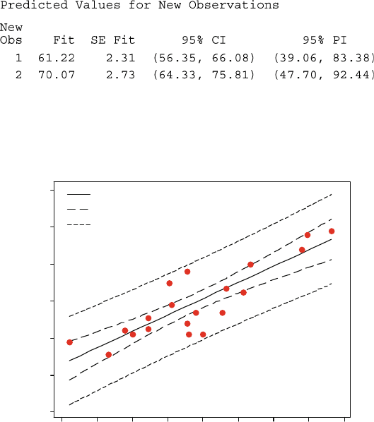
Figure 12.21 shows MINITAB output resulting from a request to calculate

confidence interv als for the mean graduation rate when the SAT is 1100 and 1200.

Because this optional output was requested, the confidence intervals (Figure 12.21)

were appended to the bottom of the regression output given in Figure 12.19. Note

that the first interval is narrower than the second, because 1100 is much closer to

than is 1200. Figure 12.22 shows curves corr esponding to the confidence limits for

each different x value. Notice how the curves get farther and farther apart as x

moves away from

x. The output labeled PI in Figure 12.21 and the curves labeled PI

in Figure 12.22 refer to prediction intervals, to be discussed shortly.

656 CHAPTER 12 Regression and Correlation

In some situations, a CI is desired not just for a single x value but for two or

more x values. Suppose an investigator wishes a CI both for m

Yn

and for m

Yw

where

v and w are two different values of the independent variable. It is tempting to

compute the interv al (12.7) first for x ¼ v and then for x ¼ w. Suppose we use

a ¼ .05 in each computation to get two 95% intervals. Then if the variables

involved in computing the two intervals were independent of each o ther, the joint

confidence coefficient would be (.95) • (.95)  .90.

Unfortunately, the intervals are not independent because the same

, and

S are used in each. We therefore cannot assert that the joint confidence level for the

two intervals is exactly 90%. However, Exercise 79 of Chapter 8 derives the

Bonferroni inequality showing that, if the 100(1  a)% CI (12.7) is computed

both for x ¼ v and for x ¼ w to obtain joint CIs for m

Yn

and m

Yw

, then the joint

confidence level on the resulting pair of intervals is at least 100(1  2a)%. In

particular, using a ¼ .05 results in a joint confidence level of at least 90%, whereas

using a ¼ .01 results in at least 98% confidence. For example, in Example 12.15 a

95% CI for m

Y1100

was (56.35 , 66.08) and a 95% CI for m

Y1200

was (64.33, 75.81).

The simultaneous or joint confidence level for the two statements 56.35 < m

Y1100

66.08 and 64.33 < m

Y1200

< 75.81 is at least 90%.

SAT

Graduation Rate

150014001300120011001000900800700

120

100

Regression

95% CI

95% PI

Figure 12.22 MINITAB scatter plot with conﬁdence intervals and prediction

intervals for the data of Example 12.15 ■

Figure 12.21 MINITAB regression output for the data of Example 12.15

12.4 Inferences Concerning m

Y x



and the Prediction of Future Y Values 657