Devore J.L., Berk K.N. Modern Mathematical Statistics with Applications

Подождите немного. Документ загружается.

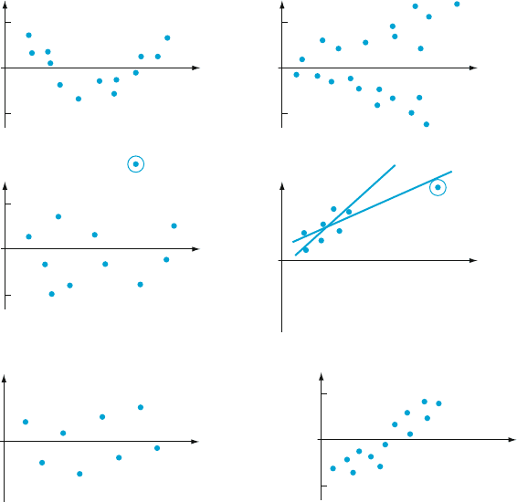
Figure 12.28 presents residual plots corresponding to items 1–3, 5, and 6. In

Chapter 4, we discussed patterns in normal probability plots that cast doubt on the

assumption of an underlying normal distribution. Notice that the residuals from the

data in Figure 12.28d with the circled point included would not by themselves

necessarily suggest further analysis, yet when a new line is fit with that point

deleted, the new line differs considerably from the original line. This type of

behavior is more difficult to identify in multiple regression. It is most likely to

arise when there is a single (or very few) data point(s) with independent variable

value(s) far removed from the remainder of the data.

We now indicate briefly what remedies are available for the types of diffi-

culties. For a more comprehensive discussion, one or more of the references on

regression analysis should be consulted. If the residual plot looks something like

that of Figure 12.28a, exhibiting a curved pattern, then a nonlinear function of x

may be fit.

The residual plot of Figure 12.28b suggests that, although a straight-line

relationship may be reasonable, the assumption that V(Y

) ¼ s

for each i is of

doubtful validity. When the error term e satisfies the independence and constant

variance assumptions (normality is not needed) for the simple linear regression

-2

e* e*

Time order

of observation

Omitted

independent

variable

Figure 12.28 Plots that indicate abnormality in data: (a) nonlinear relationship;

(b) non-constant variance; (c) discrepant observation; (d) observation with large

inﬂuence; (e) dependence in errors; (f) variable omitted

678

CHAPTER 12 Regression and Correlation

model of Section 12.1, it can be shown that among all unbiased estimators of b

and

, the ordinary least squares estimators have minimum variance. These estimators

give equal weight to each (x

, Y

). If the variance of Y increases with x, then Y

’s for

large x

should be given less weight than those with small x

. This suggests that

and b

should be estimated by minimizing

ðb

; b

Þ¼

½y

ðb

þ b

Þ

ð12:15Þ

where the w

’s are weights that decrease with increasing x

. Minimization of

Expression (12.15 ) yields weighted least squares estimates. For example, if the

standard deviation of Y is proportional to x (for x > 0)—that is, V(Y) ¼ kx

—then

it can be shown that the weights w

¼ 1=x

yield minimum variance estimators of

and b

. The books by Michael Kutner et al. and by S. Chatterjee et al. contain

more detail (see the chapter bibliography). Weighted least squares is used quite

frequently by econometricians (economists who use statistical methods) to estimate

parameters.

When plots or other evidence suggest that the data set contains outliers or

points having large influence on the resulting fit, one possible approach is to omit

these outlying points and recompute the estimated regression equation. This would

certainly be correct if it were found that the outliers resulted from errors in

recording data values or experimental errors. If no assignable cause can be found

for the outliers, it is still desirable to report the estimated equation both with and

without outliers. Yet another approach is to retain possible outliers but to use an

estimation principle that puts relatively less weight on outlying values than does the

principle of least squares. One such principle is MAD (minimize absolute devia-

tions), which selects

and

to minimize

 b

þ b

ðÞ

. Unlike the

estimates of least squares, there are no nice formulas for the MAD estimates;

their values must be found by using an iterative computational procedure . Such

procedures are also used when it is suspected that the e

’s have a distribution that is

not normal but instead has “heavy tails” (making it much more likely than for the

normal distribution that discrepant values will enter the sample); robust regression

procedures are those that produce reliable estimates for a wide variety of underly-

ing error distributions. Least squares estimators are not robust in the same way that

the sample mean

X is not a robust estimator for m.

When a plot suggests time dependence in the error terms, an appropriate

analysis may involve a transformation of the y’s or else a model explicitly including

a time variable. Lastly, a plot such as that of Figure 12.28f, which shows a pattern in

the residuals when plotted against an omitted variable, suggests considering a

model that includes the omitted variable. We have already seen an illustration of

this in Example 12.24. ■

Exercises Section 12.6 (68–77)

68. Suppose the variables x ¼ commuting distance

and y ¼ commuting time are related according

to the simple linear regression model with

s ¼ 10.

a. If n ¼ 5 observations are made at the x values

¼ 5, x

¼ 10, x

¼ 15, x

¼ 20, and

¼ 25, calculate the standard deviations of

the five corresponding residuals.

b. Repeat part (a) for x

¼ 5, x

¼ 10, x

¼ 15,

¼ 20, and x

¼ 50.

c. What do the results of parts (a) and (b) imply

about the deviation of the estimated line from

12.6 Assessing Model Adequacy 679

the observation made at the largest sampled x

value?

69. The x values and standardized residuals for the

chlorine flow/etch rate data of Exercise 51 (Sec-

tion 12.4) are displayed in the accompanying

table. Construct a standardized residual plot and

comment on its appearance.

x 1.50 1.50 2.00 2.50 2.50

e* .31 1.02 1.15 1.23 .23

x 3.00 3.50 3.50 4.00

e* .73 1.36 1.53 .07

70. Example 12.7 presented the residuals from a

simple linear regression of moisture content y

on filtration rate x.

a. Plot the residuals against x. Does the resulting

plot suggest that a straight-line regression

function is a reasonable choice of model?

Explain your reasoning.

b. Using s ¼ .665, compute the values of the

standardized residuals. Is e

*  e

/s for

i ¼ 1, ..., n, or are the e

*’s not close to

being proportional to the e

’s?

c. Plot the standardized residuals against x.

Does the plot differ significantly in general

appearance from the plot of part (a)?

71. Wear resistance of certain nuclear reactor compo-

nents made of Zircaloy-2 is partly determined by

properties of the oxide layer. The following data

appears in an article that proposed a new nonde-

structive testing method to monitor thickness of

the layer (“Monitoring of Oxide Layer Thickness

on Zircaloy-2 by the Eddy Current Test Method,”

J. Test. Eval., 1987: 333–336). The variables are

x ¼ oxide-layer thickness (mm) and y ¼ eddy-

current response (arbitrary units).

x 0 7 17 114 133

y 20.3 19.8 19.5 15.9 15.1

x 142 190 218 237 285

y 14.7 11.9 11.5 8.3 6.6

a. The authors summarized the relationship by

giving the equation of the least squares line as

y ¼ 20.6  .047x. Calculate and plot the resi-

duals against x and then comment on the

appropriateness of the simple linear regres-

sion model.

b. Use s ¼ .7921 to calculate the standardized

residuals from a simple linear regression.

Construct a standardized residual plot and

comment. Also construct a normal probability

plot and comment.

72. As the air temperature drops, river water

becomes supercooled and ice crystals form.

Such ice can significantly affect the hydraulics

of a river. The article “Laboratory Study of

Anchor Ice Growth” (J. Cold Regions Engrg.,

2001: 60–66) described an experiment in which

ice thickness (mm) was studied as a function of

elapsed time (hr) under specified conditions. The

following data was read from a graph in the

article: n ¼ 33; x ¼ .17, .33, .50, .67, ..., 5.50;

y ¼ .50, 1.25, 1.50, 2.75, 3.50, 4.75, 5.75, 5.60,

7.00, 8.00, 8.25, 9.50, 10.50, 11.00, 10.75, 12.50,

12.25, 13.25, 15.50, 15.00, 15.25, 16.25, 17.25,

18.00, 18.25, 18.15, 20.25, 19.50, 20.00, 20.50,

20.60, 20.50, 19.80.

a. The r

value resulting from a least squares fit

is .977. Given the high r

, does it seem appro-

priate to assume an approximate linear rela-

tionship?

b. The residuals, listed in the same order as the x

values, are

1.03 0.92 1.35 0.78 0.68 0.11 0.21

0.59 0.13 0.45 0.06 0.62 0.94 0.80

0.14 0.93 0.04 0.36 1.92 0.78 0.35

0.67 1.02 1.09 0.66 0.09 1.33 0.10

0.24 0.43 1.01 1.75 3.14

Plot the residuals against x, and reconsider the

question in (a). What does the plot suggest?

73. The accompanying data on x ¼ true density

(kg/mm

) and y ¼ moisture content (% d.b.)

was read from a plot in the article “Physical

Properties of Cumin Seed” (J. Agric. Engrg.

Res., 1996: 93–98).

x 7.0 9.3 13.2 16.3 19.1 22.0

y 1046 1065 1094 1117 1130 1135

The equation of the least squares line is y

¼ 1008.14 + 6.19268x (this differs very slightly

from the equation given in the article); s ¼ 7.265

and r

¼ .968.

a. Carry out a test of model utility and comment.

b. Compute the values of the residuals and

plot the residuals against x. Does the plot

suggest that a linear regression function is

inappropriate?

680

CHAPTER 12 Regression and Correlation

c. Compute the values of the standardized

residuals and plot them against x. Are there

any unusually large (positive or negative)

standardized residuals? Does this plot give

the same message as the plot of part (b)

regarding the appropriateness of a linear

regression function?

74. Continuous recording of heart rate can be used to

obtain information about the level of exercise

intensity or physical strain during sports partici-

pation, work, or other daily activities. The article

“The Relationship Between Heart Rate and Oxy-

gen Uptake During Non-Steady State Exercise”

(Ergonomics, 2000: 1578–1592) reported on a

study to investigate using heart rate response (x,

as a percentage of the maximum rate) to predict

oxygen uptake (y, as a percentage of maximum

uptake) during exercise. The accompanying data

was read from a graph in the paper.

HR 43.5 44.0 44.0 44.5 44.0 45.0 48.0 49.0

22.0 21.0 22.0 21.5 25.5 24.5 30.0 28.0

HR 49.5 51.0 54.5 57.5 57.7 61.0 63.0 72.0

32.0 29.0 38.5 30.5 57.0 40.0 58.0 72.0

Use a statistical software package to perform a

simple linear regression analysis. Considering

the list of potential difficulties in this section,

see which of them apply to this data set.

75. Consider the following four (x, y) data sets; the

first three have the same x values, so these values

are listed only once (Frank Anscombe, “Graphs in

Statistical Analysis,” Amer. Statist., 1973: 17–21):

1–312344

xyyyxy

10.0 8.04 9.14 7.46 8.0 6.58

8.0 6.95 8.14 6.77 8.0 5.76

13.0 7.58 8.74 12.74 8.0 7.71

9.0 8.81 8.77 7.11 8.0 8.84

11.0 8.33 9.26 7.81 8.0 8.47

14.0 9.96 8.10 8.84 8.0 7.04

6.0 7.24 6.13 6.08 8.0 5.25

4.0 4.26 3.10 5.39 19.0 12.50

12.0 10.84 9.13 8.15 8.0 5.56

7.0 4.82 7.26 6.42 8.0 7.91

5.0 5.68 4.74 5.73 8.0 6.89

For each of these four data sets, the values of the

summary statistics

, and

are virtually identical, so all quantities

computed from these five will be essentially

identical for the four sets—the least squares

line (y ¼ 3 + .5x), SSE, s

, r

, t intervals, t sta-

tistics, and so on. The summary statistics provide

no way of distinguishing among the four data

sets. Based on a scatter plot and a residual plot

for each set, comment on the appropriateness or

inappropriateness of fitting a straight-line model;

include in your comments any specific sugges-

tions for how a “straight-line analysis” might be

modified or qualified.

76. a. Express the ith residual Y



(where

) in the form

, a linear

function of the Y

’s. Then use rules of vari-

ance to verify that VðY



Þ is given by

Expression (12.13).

b. As x

moves farther away from x, what hap-

pens to Vð

Þ and to VðY



Þ?

77. If there is at least one x value at which more than

one observation has been made, there is a formal

test procedure for testing

: m

Y·x

¼ b

+ b

x for some values b

, b

(the

true regression function is linear)

versus

: H

is not true (the true regression function is

not linear)

Suppose observations are made at x

, x

, ..., x

Let Y

; Y

; ...; Y

denote the n

observations

when x ¼ x

; ...; Y

; Y

; ...; Y

denote the n

observations when x ¼ x

.Withn ¼ Sn

(the

total number of observations), SSE has n  2df.

We break SSE into two pieces, SSPE (pure error)

and SSLF (lack of fit), as follows:

SSPE ¼

ðY

 Y

i



ðY

i

SSLF ¼ SSE  SSPE

The n

observations at x

contribute n

 1dfto

SSPE, so the number of degrees of freedom for

SSPE is S

 1) ¼ n  c and the degrees of

freedom for SSLF is n 2  (n c) ¼ c 2. Let

MSPE ¼ SSPE/(n  c), MSLF ¼ SSLF/(c  2).

Then it can be shown that whereas E(MSPE) ¼ s

whether or not H

is true, E(MSLF) ¼ s

if H

true and E(MSLF) > s

if H

is false.

Test statistic: F ¼ MSLF=MSPE

Rejection region: f  F

;c2;nc

12.6 Assessing Model Adequacy 681

The following data comes from the article

“Changes in Growth Hormone Status Related to

Body Weight of Growing Cattle” (Growth, 1977:

241–247), with x ¼ body weight and y ¼ meta-

bolic clearance rate/ body weight.

x 110 110 110 230 230 230 360

y 235 198 173 174 149 124 115

x 360 360 360 505 505 505 505

y 130 102 95 122 112 98 96

(So c ¼ 4, n

¼ n

¼ 3, n

¼ n

¼ 4.)

a. Test H

versus H

at level .05 using the lack-

of-fit test just described.

b. Does a scatter plot of the data suggest that the

relationship between x and y is linear? How

does this compare with the result of part (a)?

(A nonlinear regression function was used in

the article.)

12.7

Multiple Regression Analysis

In multiple regression, the objective is to build a probabilistic model that relates a

dependent variable y to more than one independent or predictor variable. Let k

represent the number of predictor variables (k  2) and denote these predictors by

, x

, ..., x

. For example, in attempting to predict the selling price of a house, we

might have k ¼ 3withx

¼ size (ft

), x

¼ age (years), and x

¼ number of rooms.

DEFINITION

The general additive multiple regression model equation is

Y ¼ b

þ b

þþb

þ e ð12:16Þ

where E(e) ¼ 0 and V(e) ¼ s

. In addition, for purposes of testing hypoth-

eses and calculating CIs or PIs, it is assumed that e is normally d istributed and

also that the e’s associated with various observations, and thus the Y

’s

themselves, are independent of one another.

Let x



; x



; ...; x



be particular values of x

, ..., x

. Then (12.16 ) implies that

Yx



;...;x



¼ b

þ b



þþb



ð12:17Þ

Thus, just as b

+ b

x describes the mean Y value as a function of x in simple linear

regression, the true (or population) regression function b

+ b

+  + b

gives the expected value of Y as a function of x

, ..., x

.Theb

’s are the true (or

population) regression coefficients. The regression coefficient b

is interpreted as

the expected change in Y associated with a 1-unit increase in x

while x

, ..., x

are

held fixed. Analogous interpretations hold for b

, ..., b

Estimating Parameters

The data in simple linear regression consists of n pairs (x

, y

), ...,(x

, y

). Suppose

that a multiple regression model contains two predictor variables, x

and x

. Then

each observation will consist of three numbers (a triple): a value of x

, a value of x

and a value of y. More generally, with k independent or predictor variables, each

682 CHAPTER 12 Regression and Correlation

observation will consist of k + 1 numbers (a “k + 1 tuple”). The values of the

predictors in the individual observations are denoted using double-subscripting:

¼ the value of the jth predictor x

in the ith observation

i ¼ 1; ... ; n; j ¼ 1; ... ; kðÞ:

Thus the first subscript is the observation number and the second subscript is the

predictor number. For example, x

is the value of the 3rd predictor in the 8th

observation (to avoid confusion, a comma can be inserted between the two sub-

scripts, e.g. x

12,3

). The first observation in our data set is then (x

, x

, ..., x

, y

the second is (x

, x

, ..., x

, y

), and so on.

Consider candidates b

, b

, ..., b

for estimates of the b

’s and the

corresponding candidate regression function b

+ b

+  + b

. Substituting

the predictor values for any individual observation into this candidate function

gives a predict ion for the y value that would be observed, and subtracting this

prediction from the actual observed y value gives the prediction error. The princi-

ple of least squares says we should square these prediction errors, sum, and then

take as the least squares estimates

;

; ...;

, the values of the b

’s that minimize

the sum of squared prediction errors. To carry out this program, form the criterion

function (sum of squared prediction errors)

gðb

; b

; ...; b

Þ¼

i¼1

 b

þ b

þþb

ðÞ½

and then take the partial derivative of g(·) with respect to each b

(j ¼ 0, 1, ..., k),

and equate these k + 1 partial derivatives to 0. The result is a system of k +1

equations, the normal equations, in the k + 1 unknowns (the b

’s). It is very

important here that the normal equations are linear in the unknowns becau se the

criterion function is quadratic.



þþ



þþ



þþ

i;k1



k1



We will assume that the system has a unique solution, the least squares estimates

;

; ...;

. The next section uses matrix algebra to deal with the system of

equations and develop inferential procedures for multiple regression. For the

moment, though, we shall take advantage of the fact that all of the commonly

used statistical software packages are programmed to solve the equations and

provide the results needed for inference.

Sometimes interest in the individual regression coefficients is the main

reason for doing the regression. The article “Autoregressive Modeling of Baseball

Performance and Salary Data,” Proceedings of the Statistical Graphics Section,

American Statistical Association, 1988, 132–137, describes a multiple regression of

runs scored as a function of singles, doubles, triples, home runs, and walks

(combined with hit-by-pitcher). The estimated regression equation is

12.7 Multiple Regression Analysis 683

runs ¼2:49 þ :47 singles þ :76 doubles þ 1: 14 triples þ 1:54 home runs

þ :39 walks

This is very similar to the popular slugging percentage statistic, which gives

weight 1 to singles, 2 to doubles, 3 to triples, and 4 to home runs. However, the

slugging percentage gives no weight to walks, whereas the regression puts weight

.39 on walks, more than 80% of the weight it assigns to singles. The importance of

walks is well-known among statisticians who follow baseball, and it is interesting

that there are now some statistically savvy people in major league baseball man-

agement who are emphasizing walks in choosing players.

Example 12.25 The article “Factors Affecting Achievement in the First Course in Calculus”

(J. Exper. Educ., 1984: 136–140) discussed the ability of several variables to

predict y ¼ freshman calculus grade (on a scale of 0–100). The variables included

¼ an algebra placement test given in the first week of class, x

¼ ACT math

score, x

¼ ACT natural science score, and x

¼ high school percentile rank. Here

are the scores for the first five and the last five of the 80 students (the data set is

available from the web site for this book):

Observation Algebra ACTM ACTNS HS Rank Grade

12127236862

21629329975

32230329895

42534289078

52229239995

76 22 29 26 88 85

77 17 29 33 92 75

78 26 27 29 95 88

79 26 28 30 99 95

80 21 28 30 99 85

The JMP statistical computer package gave the following least squares estimates:

¼ 36:12

¼ :9610

¼ :2718

¼ :2161

¼ :1353

Thus we estimate that .9610 is the average increase in final grade associated with a

1–point increase in the algebra placement score when the other three predictors are

held fixed. Another way to interpret this is to say that a 10-point increase in the algebra

pretest score, with the other scores held fixed, corresponds to a 9.6 point increase in the

final grade, an increase of approximately one letter grade if A ¼ 90s, B ¼ 80s, etc.

The other estimated coefficients are interpreted in a similar manner.

The estimated regression equation is

y ¼ 36:12 þ :9610x

þ :2718x

þ :2161x

þ :1353x

A point prediction of final grade for a single student with an algebra test score of 25,

ACTM score of 28, ACTNS score of 26, and a high school percentile rank of 90 is

y ¼ 36:12 þ :9610 25ðÞþ:2718 28ðÞþ:2161 26ðÞþ:1353 90ðÞ¼85:55

684 CHAPTER 12 Regression and Correlation

a middle B. This is also a point estimate of the mean for the population of all

students with an algebra test score of 25, ACTM score of 28, ACTNS score of 26,

and a high school percentile rank of 90

■

and the Coefﬁcient of Multiple Determination

Substituting the values of the predictors from the successive observations into the

equation for an estimated regression function gives the predicte d or fitted values

;

; ...;

. For example, since the values of the four predictors for the last

observation in Example 12.25 are 21, 28, 30, and 99, respectively, the

corresponding predicted value is

¼ 83:79. The residuals are the differences



; ...; y



. In simple linear regression, they were the vertical deviations

from the least squares line, but in general there is no geometric interpretation in

multiple regression (the exception is the case k ¼ 2, where the estimated regression

function specifies a plane in three dimensions and the residuals are the vertical

deviations from the plane). The last residual in Example 12.25 is 85 

83.79 ¼ 1.21. The closer the residuals are to 0, the better the job our estimated

equation is doing in predicting the y values actually observed.

The residuals are sometimes important not just for judging the quality of a

regression. Several enterprising students developed a multiple regression model

using age, size in square feet, etc. to predict the price of four-unit apartment

buildings. They found that one building had a strongly negative residua l, meaning

that the price was much lower than predicted. As it turned out, the reason was that

the owner had “cash-flow” problems, and needed to sell quickly, so the students got

an unusually good deal.

As in simple linear regression, the estimate of the variance parameter s

based on the sum of squared residuals (or sum of squared errors) SSE = Sðy



Previously, we divided SSE by n  2 to obtain the estimate. The explanation was that

the two parameters

and

had to be estimated, entailing a loss of two degrees of

freedom. For each parameter there is a normal equation that can be expressed as a

constraint on the residuals, with a loss of 1 df. In multiple regression with k

predictors, k + 1 df are lost in estimating the b

’s (don’t forget the constant term

). Here are the normal equations rewritten as constraints on the residuals:

½y

ðb

þ x

þþx

Þ ¼ 0

½y

ðb

þ x

þþx

Þ ¼ 0

½y

ðb

þ x

þþx

Þ ¼ 0

The first equation says that the sum of the residuals is 0, the second equation

says that the first predictor times the residual sums to 0, etc. These k + 1 constraints

allow any k + 1 residuals to be determined from the others. This implies that SSE is

based on n  (k + 1) df and this is the divisor in the estimate of s

¼ s

SSE

n ðk þ 1Þ

¼ MSE;

s ¼ s ¼

ﬃﬃﬃﬃ

12.7 Multiple Regression Analysis 685

SSE can once again be regarded as a measure of unexplained variation in the

data—the extent to which observed variation in y cannot be attributed to the model

relationship. Total sum of squares SST, defined as

ðy

 yÞ

as in simple linear

regression, is a measure of total variation in the observed y values. Taking the ratio

of these sums of squares and subtracting from one gives the coefficient of multiple

determination

¼ 1 

SSE

SST

Sometimes called just the coefficient of determination or the squared multiple

correlation, R

is interpreted as the proportion of observed variation that can be

attributed to, or equivalently, explained by, the model relationship. Thinking of

SST as the error sum of squares using just the constant model (with b

as the only

term in the model) havi ng

y as the predictor, R

is the proportion by which the

model reduces the error sum of squares. For example, if SST ¼ 20 and SSE ¼ 5,

then the model reduces the error sum of squares by 75%, so R

¼ .75. The closer R

is to 1, the greater the proportion of observed variation that can be explained by the

fitted model.

Unfortunately, there is a potential problem with R

: its value can be inflated

by including predictors in the model that are relatively unimportant or even

frivolous. For example, suppose we plan to obtain a sample of 20 recently sold

houses in order to relate sale price to various characteristics of a house. Natural

predictors include interior size, lot size, age, number of bedrooms, and distance to

the nearest school. Suppose we also include in the model the diameter of the

doorknob on the door of the master bedroom, the height of the toilet bowl in the

master bath, and so on until we have 19 predict ors. Then unless we are extrem ely

unlucky in our choice of predictors, the value of R

will be 1 (because 20

coefficients are estimated from 20 observations)! Rather than seeking a model

that has the highest possibl e R

value, which can be achieved just by “pack ing” our

model with predictors, what is desired is a relatively simple model based on just a

few important predictors whose R

value is high.

It is therefore desirable to adjust R

to take account of the fact that its value

may be quite high just because many predictors were used relative to the amount of

data. The adjusted coefficient of multiple determination is defined by

¼ 1 

MSE

MST

¼ 1 

SSE=½n ðk þ 1Þ

SST=ðn  1Þ

¼ 1 

n  1

n ðk þ 1Þ

SSE

SST

The ratio multiplying SSE/SST in adjusted R

exceeds 1 (the denominator is

smaller than the numerator), so adju sted R

is smaller than R

itself, and in fact

will be much smaller when k is large relative to n. A value of R

much smaller than

is a warning flag that the chosen model has too many predictors relative to the

amount of data.

Example 12.26 Continuing with the previous example in which a model with four predictors was fit

to the calculus data consisting of 80 observations, the JMP software package gave

SSE ¼ 7346.05 and SST ¼ 10,332.20, from which s ¼ 9.90, R

¼ .289, and

¼ :251. The estimated standard deviation s is very close to 10, which corre-

sponds to one letter grade on the usual A ¼ 90s, B ¼ 80s, ..., scale. About 29% of

686 CHAPTER 12 Regression and Correlation

observed variation in grade can be attributed to the chosen model. The difference

between R

and R

is not very dramatic, a reflection of the fact that k ¼ 4 is much

smaller than n ¼ 80.

■

A Model Utility Test

In multiple regression, is there a single indicator that can be used to judge whether a

particular model will be useful? The value of R

certainly communicates a prelimi-

nary message, but this value is sometimes deceptive because it can be greatly

inflated by using a large number of predictors (large k) relative to the sample size n

(this is the rationale behind adjusting R

The model utility test in simple linear regression involved the null hypothesis

: b

¼ 0, according to which there is no useful relation between y and the single

predictor x. Here we consi der the assertion that b

¼ 0, b

¼ 0, ..., b

¼ 0, which

says that there is no useful relationship between y and any of the k predictors. If at

least one of these b’s is not 0, the corresponding predictor(s) is (are) useful. The test

is based on a statistic that has a particular F distribution when H

is true (see

Sections 10.5 and 11.1 for more about F tests).

Null hypothesis: H

: b

¼ b

¼¼b

¼ 0

Alternative hypothesis: H

: at least one b

6¼ 0 i ¼ 1; ...; kðÞ

Test statistic value:

f ¼

ð1  R

Þ=½n ðk þ 1Þ

SSR=k

SSE/½n ðk þ 1Þ

MSR

MSE

ð12:18Þ

where SSR ¼ regression sum of squares ¼ SST  SSE

Rejection regio n for a level a test: f  F

a,k,n(k+1)

See the next section for an explanation of why the ratio MSR/MSE has an F

distribution under the null hypothesis.

Except for a constant multiple, the test statistic here is R

/(1  R

), the ratio

of explained to unexplained variation. If the proportion of explained variation is

high relative to unexplained, we would naturally want to reject H

and confirm the

utility of the model. However, the factor [n  (k + 1)]/k decreases as k increases,

and if k is large relative to n, it will reduce f considerably.

Example 12.27 Re turning to the calculus data of Example 12.25, a model with k ¼ 4 predictors

was fitted, so the relevant hypotheses are

: b

¼ b

¼ 0

: at least one of these four b’s is not 0

Figure 12.29 shows output from the JMP statist ical package. The values of s (Root

Mean Square Error), R

, and adjusted R

certainly suggest a useful model. The

value of the model utility F ratio is

f ¼

ð1  R

Þ=½n ðk þ 1Þ

:289=4

:711=ð80  5Þ

¼ 7:62

12.7 Multiple Regression Analysis 687