Devore J.L., Berk K.N. Modern Mathematical Statistics with Applications

Подождите немного. Документ загружается.

y ¼ X

b ¼ X½X

X

1

Because y-hat is the product of H ¼ X½X

X

1

and y, the matrix H is called the

hat matrix. A residual is y



, so the vector of n residuals is

y 

y ¼ y  Hy ¼ðI  HÞy:

The error sum of squares SSE is the sum of the n squared residuals,

SSE = (y 

yÞ

ðy 

yÞ¼ y 

An unbiased estimator of s

is MSE ¼ S

¼ SSE/[n  (k + 1)]. Notice that the

estimated variance is the average [with n  (k + 1) in place of n] squared residual.

The divisor n  (k + 1) is used because SSE is proportional to a chi-square rv with

n  (k + 1) degrees of freedom under the assumptions given at the beginnin g of this

section, including the assumption that X

X be invertible.

We can rewrite the normal equations in the form

0 ¼ X

y  X

b ¼ X

ðy  X

bÞ¼X

ðy 

yÞ: ð12:19Þ

Because the transpose of X times the residual vector is zero, each of the columns of

X, including the column of 1’s, is perpendicular to the residual vector y 

y.In

particular, because the dot product of the column of 1’s with the residual vector is

zero, the sum of the residuals is zero. There are k + 1 columns of X, and the dot

product of each column with the residual vector is zero, so there are k + 1 condi-

tions satisfied by the residual vector. This helps to explain intuitively why there are

only n  (k + 1) degrees of freedom for SSE.

Letting

y be the vector with n identical components y, the total sum of

squares SST is the sum of the squared deviations from

y, SST ¼ y  y

. Simi-

larly, the regression sum of squares SSR is defined to be the sum of the squared

deviations of the predicted values from

y, SSR ¼

y  y

. As before the ANOVA

relationship is

SST ¼ SSE þ SSR ð12:20Þ

This can be obtained by subtracting and adding

SST ¼jjy 

yjj

¼½ðy 

yÞþð

y  yÞ

½ðy 

yÞþð

y  yÞ

¼jjy 

yjj

þjj

y  yjj

¼ SSE þ SSR:

The cross-terms in the matrix product are zero because of Equation (12.19) (see

Exercise 102).

Recall that the null hypothesis in the model utility test is H

: b

¼¼b

¼0,

in which case the model consists of just b

. That is, under H

the observations all have

the same mean m ¼ b

. For a normal random sample with mean m and standard

708 CHAPTER 12 Regression and Correlation

deviation s, a proposition in Section 6.4 shows that SST/s

has the chi-squared

distribution with n  1 df. Dividing Equation (12.20) by s

gives

SST

SSE

SSR

It can be shown that SSE and SSR are independent of each other. We know that

SST=s

 w

n1

under the null hypothesis and SSE=s

 w

nk1

. Then, by a prop-

osition in Section 6.4, SSR/s

is distributed as chi-squared with degrees of freedom

[n  1]  [n  (k + 1)] ¼ k. Recall from Section 6.4 that the F distribution is the

ratio of two independent chi-squares that have been divided by their degrees of

freedom. Applying this to SSR/s

and SSE/s

leads to the F ratio

SSR

SSE

½n ðk þ 1Þ

SSR

SSE

n ðk þ 1Þ

MSR

MSE

 F

k;nðkþ1Þ

ð12:21Þ

Here MSR ¼ SSR/k and MSE was previously defined as SSE/[n  (k + 1)]. The

F ratio MSR/MSE is a standard part of regression output for statistical computer

packages. It tests the null hypothesis H

: b

¼  ¼ b

¼ 0, the hypothesis of a

constant mean model. This is the model utility test, and it tests the hypothesis that

the explanatory variables are useless for predicting y. Rejection of H

occurs for

large values of the F ratio. This should be intuitively reasonable, because if the

prediction quality is good, then SSE should be small and SSR should be large, and

therefore the F ratio should be large. The dividing line between large and small is

set using the upper tail of the F distribution. In particular, H

is typically rejected if

the F ratio exceeds F

.05,k,n(k+1)

Another measure of the relationship between y and the predictors is the R

statistic, the coefficient of multiple determination, which is the fraction SSR/SST:

SSR

SST

SST  SSE

SST

¼ 1 

SSE

SST

ð12:22Þ

By the analysis of variance, Equation (12.20), this is always between 0 and 1. The

statistic is also called the squared multiple correlation. For example, suppose

SST ¼ 200, SSR ¼ 120, and therefore SSE ¼ 80. Then R

¼ 1  (SSE/SST) ¼

1  80/200 ¼ .60, so the error sum of squares is 60% less than the total sum of

squares. This is sometimes interpreted by saying that the regression explains 60%

of the variability of y, which means that the regression has reduced the error sum of

squares by 60% from what it would be (SST) with just a constant model and no

predictors.

The F ratio and R

are equivalent statistics in the sense that one can be

obtained from the other. For example, dividing numerator and denominator through

by SST in Equation (12.21) and usin g Equation (12.22), we find that the F ratio is

[see Equation (12.18)]

F ¼

ð1  R

Þ=½n ðk þ 1Þ

12.8 Regression with Matrices 709

In the special case of just one predictor, k ¼ 1, F ¼ (n  2)R

/(1  R

), and the

multiple correlation is just the absolute valu e of the ordinary correlation coefficient.

This F is the square of the statistic T ¼

ﬃﬃﬃﬃﬃﬃﬃﬃﬃﬃﬃ

n  2

ﬃﬃﬃﬃﬃﬃﬃﬃﬃﬃﬃﬃﬃﬃ

1  R

given in Section 12.5.

Example 12.33

(Example 12.32

continued)

The predicted values and residuals are easily obtained:

y ¼ X

b ¼

120

121

12:50

12:51

130

131

61:417

95:50

129:583

162:583

177:333

210:333

225:083

258:083

y 

y ¼

132

167

170

204

230

260



129:583

162:583

177:333

210:333

225:083

258:083

2:417

4:417

7:333

6:333

4:917

1:917

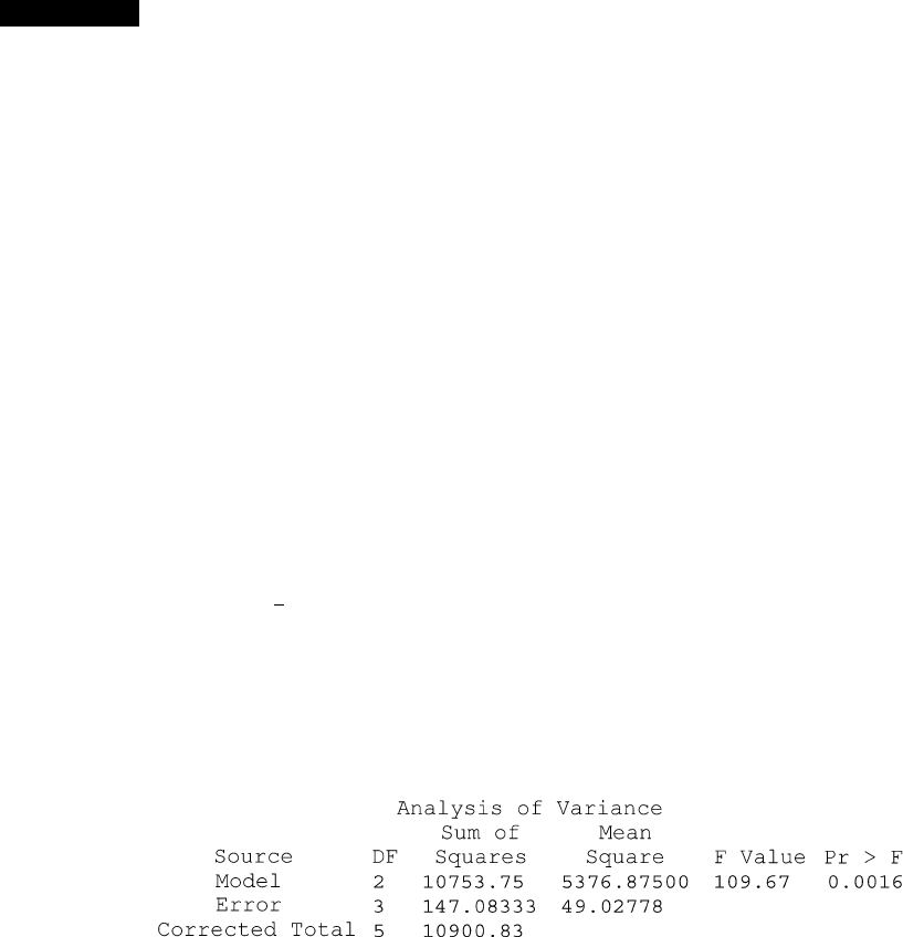
Therefore, the error sum of squares is SSE ¼ y 

¼ 2:417

þþ1:917

147:083 and MSE ¼ s

¼ SSE/[n  (k + 1)] ¼ 147.083/[6  (2 + 1)] ¼ 49.028.

The square root of this yields the estimated standard deviation s ¼ 7.002, which is

a form of average for the magnitude of the residuals. However, notice that only one

of the six residuals exceeds s in magnitude. The total sum of squares is

SST ¼jjy 

yjj

ðy

 193:83Þ

¼ 10;900:83. The regression sum of squares

can be obtained by subtraction using the analysis of variance, SSR ¼ SST 

SSE ¼ 10,900.83  147.083 ¼ 10,753.75. The sums of squares and the computa-

tion of the F test and R

are often done through an analysis of variance table, as

copied in Figure 12.36 from SAS output.

The regression sum of squares is called the model sum of squares here. The mean

square is the sum of squares divided by the degrees of freedom, and the F value

is the ratio of mean squares. Because the P-value is less than .05, we reject the

null hypothesis (that both the engine size and fuel population coefficients are 0) at

the .05 leve l. The coefficient of multiple determination is R

¼ SSR/SST ¼

10,753.75/ 10,900.83 ¼ .9865. We say that the two predictors account for

98.65% of the variance of horsepower because the error sum of squares is reduced

by 98.65% compared to the total sum of squares.

■

Figure 12.36 Analysis of variance table from SAS

710

CHAPTER 12 Regression and Correlation

Covariance Matrices

In order to develop hypothesis tests and confidence intervals for the regression

coefficients, the standard deviations of the estimated coefficients are needed. These

can be obtained from a certain covariance matrix, a matrix with the variances on

the diagonal and the covariances in the off-diagonal eleme nts. If U is a column

vector of random variables U

, ..., U

with means m

¼ E(U

), ..., m

¼ E(U

), let

m be the vector of these n means and define

CovðUÞ¼

CovðU

Þ  CovðU

CovðU

Þ  CovðU

E½ðU

m

ÞðU

m

Þ  E½ðU

m

ÞðU

m

Þ

E½ðU

m

ÞðU

m

Þ  E½ðU

m

ÞðU

m

Þ

¼ E

m

;  ; U

m

½

;

¼Ef½U m½U m

ð12:23Þ

When n ¼ 1 this reduces to just the ordinary variance. The key to finding the

needed covariance matrix is this proposition:

PROPOSITION

If A is a matrix with constant entries and V ¼ AU, then Cov(V) ¼ ACov(U)A

Proof By the linearity of the expectation operator, E(V) ¼ E(AU) ¼ AE(U).

Then

CovðVÞ¼ E AU  E AUðÞ½AU  E AUðÞ

g¼EfA½U  EðUÞðA½U  EðUÞ½Þ



¼ E AU EðUÞ½U  EðUÞ½



¼ AE U  EðUÞ½U  EðUÞ½



¼ ACovðUÞA

■

Let’s apply the proposition to find the covariance matrix of

b. Because

b ¼½X

X

1

Y, we use A ¼½X

X

1

and U ¼ Y. The transpose of A is

¼f½X

X

1

¼ X½X

X

1

. The covariance matrix of Y is just the variance

times the n-dimensional identity matrix, that is, s

I, because the observations are

independent and all have the same variance s

. Then the proposition says

Covð

bÞ¼ACovðYÞA

¼½X

X

1

½s

IX½X

X

1

¼ s

½X

X

1

ð12:24Þ

12.8 Regression with Matrices 711

We also need to find the expected value of

Eð

bÞ¼Eð½X

X

1

YÞ¼½X

X

1

EðY Þ

¼½X

X

1

EðXb þ eÞ¼½X

X

1

Xb ¼ b

That is,

b is an unbiased estimator of b (for each i,

is unbiased for estimating b

Write the inverse matrix as ½X

X

1

¼ C ¼½c

. In particular, let

; c

; ...; c

be the diagonal elements of this inverse matrix. Then

Vð

Þ¼s

. Also,

is a linear combination of Y

, ..., Y

, which are independent

normal, so ð

 b

Þ=ðs

ﬃﬃﬃﬃﬃ

ÞNð0; 1Þ It follows that (this requires the indepen-

dence of S and the estimated regression coefficients, which we will not prove)

 b

Þ=ðS

ﬃﬃﬃﬃﬃ

Þt

nðkþ1Þ

. This leads to the confidence interval and hypothesis

test for coefficients of Section 12.7.

The 95% confidence interv al for b

 t

:025;nðkþ1Þ

ﬃﬃﬃﬃﬃ

: ð12:25Þ

We can test the hypothesis H

: b

¼ b

using the t ratio

T ¼

 b

ﬃﬃﬃﬃﬃ

 t

nðkþ1Þ

Statistical software packages usually provide output for testing H

¼ 0 against

the two-sided alternative H

: b

6¼ 0. In particular, we would reject H

in favor of

at the 5% level if |t| exceeds t

.025,n(k+1)

. Usually, with computer output there is

no need to use statistical tables for hypothesis tests because P-values for these tests

are included.

Example 12.34

(Example 12.33

continued)

For the engine horsepower scenario we found that s ¼ 7.002,

¼61:417,

¼ 95:5,

¼ 33 and [X

1

has elements c

¼ 79/12, c

¼ 1, c

¼ 2/3.

Therefore, we get these 95% confidence intervals:

t

:025;6ð2þ1Þ

ﬃﬃﬃﬃﬃﬃ

¼95:5 3:182ð7:002Þ

ﬃﬃﬃ

¼95:50 22:28 ¼½73:22 ; 117:78

t

:025;6ð2þ1Þ

ﬃﬃﬃﬃﬃﬃ

¼33 3:182ð7 :002Þ

ﬃﬃﬃﬃﬃﬃﬃﬃ

2=3

¼33 18:19 ¼½14:81; 51:19

We can also do the individual t tests for the coefficients:

 0

ﬃﬃﬃﬃﬃﬃ

95:5  0

7:002

ﬃﬃﬃ

¼ 13:64; two-tailed P-value ¼ : 0009

 0

ﬃﬃﬃﬃﬃﬃ

33  0

7:002

ﬃﬃﬃﬃﬃﬃﬃﬃ

2=3

¼ 5:77; two-tailed P-value ¼ :0103

Both of these exceed t

.025,621

¼ 3.182 in absolute value (and their P-values are

less than .05), so for both of them we reject at the 5% level the null hypothesis that

the coefficient is 0, in favor of the two-sided alternative. These conclusions are

consistent with the fact that the corresponding confidence intervals do not include

zero. Also, recall that the F test rejected at the 5% level the null hypothesis that both

coefficients are zero . As our intuition suggests, horsepower increases with engine

size and horsepower is higher when the engine requires premium fuel.

■

712 CHAPTER 12 Regression and Correlation

The Hat Matrix

The foregoing proposition can be used to find estimated standard deviations for

predicted values and residua ls. Recall that the vector of predicted values can be

obtained by multiplying the hat matrix H times the Y vector, HY ¼

Y. First, in

order to apply the proposition, let’s obtain the transpose of H. With the help of the

rules (AB)

¼ B

and (A

1

)

¼ (A

)

1

, we find that H is symmetric, H

¼ H:

¼ XX

X½

1

¼ X

ðÞ

f X

X½

1

¼ XX

X½



1

¼ XX

X½

1

¼ H:

Therefore,

Covð

YÞ¼HCovðYÞH

¼ X½X

X

1

½s

IX½X

X

1

¼ s

X½X

X

1

¼ s

ð12:26Þ

A similar calculation shows that the covariance matrix of the residuals is

CovðY 

YÞ¼s

ðI  HÞð12:27Þ

Of cours e, the true variance s

is generally unknown, so the estimate s

¼ MSE is

used instead.

Example 12.35

(Example 12.34

continued)

Continue again with the horsepower example. If residuals and predicted values are

requested from SAS, then the output includes the information in Figure 12.37.

The column labeled “Std Error Mean Predict” has the estimated standard

deviations for the predicted values and it contains the square roots of the s

H matrix

diagonal elements. The column labeled “Std Error Residual” has the estimated

standard deviations for the residuals, and it contains the square roots of the diagonal

elements of s

(I  H). The column labeled “Student Residual” is what we defined as

the standardized residual in Section 12.6. It is the ratio of the previous two col-

umns.

■

The hat matrix is also important as a measure of the influence of individual

observations. Because

y ¼ Hy,

¼ h

þ h

þþh

, and therefore

=@y

¼ h

. That is, the partial derivative of

with respect to y

is the ith

diagonal element of the hat matrix. In other words, the ith diagonal element of H

measures the influence of the ith observation on its predicted value. The diagonal

Obs Residual

Student

Residual

132.0000 129.5833 5.3479 2.4167 4.520 0.535

167.0000 162.5833 5.3479 4.4167 4.520 0.977

170.0000 177.3333 4.0426 –7.3333 5.717 –1.283

204.0000 210.3333 4.0426 –6.3333 5.717 –1.108

230.0000 225.0833 5.3479 4.9167 4.520 1.088

260.0000 258.0833 5.3479 1.9167 4.520 0.424

Dep Var

Predicted

Value

StdError

Mean Predict

StdError

Residual

Figure 12.37 Predicted values and residuals from SAS

12.8 Regression with Matrices 713

elements of H are sometimes called the leverages to indicate their influence over

the regression. An observation with very high leverage will tend to pull the

regression toward it, and its residual will tend to be small. Of course, H depends

only on the values of the predictors, so the leverage measures only one aspect of

influence. If the influence of an observation is defined in terms of the effect on the

predicted values when the observation is omitted, then an influential observation is

one that has both large leverage and a large (in absolute valu e) residual.

Example 12.36 Stude nts in a statistics class measured their height, foot length, and wingspan

(measured fingertip to fingertip with hands outstretched) in inches. Leonardo da

Vinci was aware that the wingspan tends to be very nearly the same as height. Here

in Table 12.3 are the measurements for 16 students. The last column has the

leverages for the regr ession of wingspan on height and foot length.

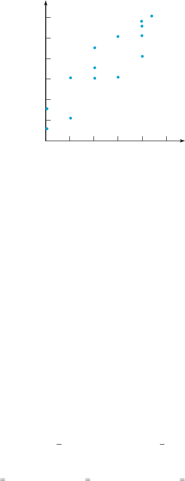
In Figure 12.38 we show the plot of height against foot length, along with the

leverage for each point. Notic e that the points at the extreme right and left of

the plot have high leverage, and the points near the center have low leverage.

However, it is interesting that the point with highest leverage is not at the extremes

of height or foot length. This is student number 7, with a 10-in. foot and height of

71 in., and the high leverage comes from the height being extreme relative to foot

length. Indeed, when there are several predictors, high leverage often occurs when

values of one predictor are extreme relative to the values of other predictors. For

example, if height and weight are predictors, then an overweight or underweight

subject would likely have high leverage.

Table 12.3 Height, foot length, and wingspan

Obs Height Foot Wingspan Leverage

1 63.0 9.0 62.0 0.239860

2 63.0 9.0 62.0 0.239860

3 65.0 9.0 64.0 0.228236

4 64.0 9.5 64.5 0.223625

5 68.0 9.5 67.0 0.196418

6 69.0 10.0 69.0 0.083676

7 71.0 10.0 70.0 0.262182

8 68.0 10.0 72.0 0.067207

9 68.0 10.5 70.0 0.187088

10 72.0 10.5 72.0 0.151959

11 73.0 11.0 73.0 0.143279

12 73.5 11.0 75.0 0.168719

13 70.0 11.0 71.0 0.245380

14 70.0 11.0 70.0 0.245380

15 72.0 11.0 76.0 0.128790

16 74.0 11.2 76.5 0.188340

714

CHAPTER 12 Regression and Correlation

In Figure 12.39 there is some useful output from MINITAB, including the

model utility test, the regression coefficients, and the correlations among the

variables. The correlation table shows all three correlations among the three vari-

ables along with their P-values. Clearly, the three variables are very strongl y

related. However, when wingspan is regressed on height and foot length, the

P-value for foot length is greater than .05, so we can consider eliminating foot

length from the regression equation. Does it make sense for foot length to be very

strongly related to wingspan, as measured by correlation, but for the foot length

term to be not statistically significant in the regression equation? The difference is

that the regression test is asking whether foot length is needed in addition to height.

Because the two predictors are themselves highly correlated, foot length is redun-

dant in the sense that it offers little prediction ability beyond what is contributed

by height.

Analysis of Variance

Source DF SS MS F P

Regression 2 294.79 147.40 67.33 0.000

Residual Error 13 28.46 2.19

Total 15 323.25

Predictor Coef SE Coef T P

Constant

6.085 8.018 0.76 0.461

height 0.8060 0.2305 3.50 0.004

foot 1.973 1.044 1.89 0.081

1.47956 R-Sq 91.2% R-Sq(adj) 89.8%

Correlations: height, foot, wingspan

height foot

foot 0.892

0.000

wingspan 0.942 0.911

0.000 0.000

Figure 12.39 Regression output for height, foot length, and wingspan ■

9.0 9.5 10.0 10.5 11.0 11.5

Height

Foot length

0.08

0.07

0.22

0.26

0.15

0.25

0.13

0.23

0.24

0.14

0.19

0.17

0.20

0.19

Figure 12.38 Plot of height and foot length showing leverage

12.8 Regression with Matrices 715

Exercises Section 12.8 (91–104)

91. Fit the model Y ¼ b

þ b

þ e to the

data

1 11

111

1 10

114

a. Determine X and y and express the normal

equations in terms of matrices.

b. Determine the

b vector, which contains the

estimates for the three coefficients in the

model.

c. Determine

y, the predictions for the four

observations, and also the four residuals.

Find SSE by summing the four squared resi-

duals. Use this to get the estimated variance

MSE.

d. Use the MSE and c

to get a 95% confidence

interval for b

e. Carry out a t test for the hypothesis H

¼ 0 against a two-tailed alternative, and

interpret the result.

f. Form the analysis of variance table and carry

out the F test for the hypothesis H

: b

¼ b

¼ 0. Find R

and interpret.

92. Consider the model Y ¼ b

þ b

þ e for the

data

.5 1

.5 2

.5 3

.5 8

.5 9

.5 7

.5 8

a. Determine the X and y matrices and express

the normal equations in terms of matrices.

b. Determine the

b vector, which contains the

estimates for the two coefficients in the

model.

c. Determine

y, the predictions for the eight

observations, and also obtain the eight resi-

duals.

d. Find SSE by summing the eight squared resi-

duals. Use this to get the estimated variance

MSE.

e. Use the MSE and c

to get a 95% confidence

interval for b

f. Carry out a t test for the hypothesis H

: b

¼ 0

against a two-tailed alternative.

g. Carry out the F test for the hypothesis H

¼ 0. How is this related to part (f)?

93. Suppose that the model consists of just

Y ¼ b

þ e so k ¼ 0. Estimate b

from

1

y. Find simple expressions for s and

, and use them along with Equation (12.25)

to express simply the 95% confidence interval

for b

. Your result should be equivalent to the

one-sample t confidence interval in Section 8.3.

94. Suppose we have (x

, y

), ...,(x

, y

). Let k ¼ 1

and let x

¼ x

 x; i ¼ 1; ...; n, so our model

is y

¼ b

þ b

ðx

 xÞþe

i ¼ 1; ...; n:

a. Obtain

and

from [X

1

b. Find c

and c

and use them to simplify the

confidence intervals [Equation (12.25)] for

and b

c. In terms of computing [X

1

, why is it better

to have x

¼ x

 x rather than x

¼ x

95. Suppose that we have Y

, ..., Y

~ N( m

m+1

, ..., Y

m+n

~ N( m

, s

), and all m + n obser-

vations are independent. These are the assump-

tions of the pooled t procedure in Section 10.2.

Let k ¼ 1, x

¼ .5, ..., x

¼ .5, x

m+1,1

¼.5,

..., x

m+n,1

¼.5. For convenience in inverting

X assume m ¼ n.

a. Obtain

and

from [X

1

b. Find simple expressions for

y, SSE, s, c

c. Use parts (a) and (b) to find a simple expres-

sion for the 95% CI [Equation (12.25)] for b

Letting

be the mean of the first m observa-

tions and

be the mean of the next n obser-

vations, your result should be

t

:025;mþn2

ﬃﬃﬃﬃﬃﬃﬃﬃﬃﬃﬃ

y

t

:025;mþn2

ﬃﬃﬃﬃﬃﬃﬃﬃﬃﬃﬃﬃﬃﬃﬃﬃﬃﬃﬃﬃﬃﬃﬃﬃﬃﬃﬃﬃﬃﬃﬃﬃﬃﬃﬃﬃﬃﬃﬃﬃﬃﬃﬃﬃﬃﬃﬃﬃﬃﬃﬃﬃﬃﬃﬃﬃﬃﬃﬃ

i¼1

ðy

y

mþn

i¼mþ1

ðy

y

m þn 2

ﬃﬃﬃﬃﬃﬃﬃﬃﬃﬃﬃ

which is the pooled variance confidence inter-

val discussed in Section 9.2.

716 CHAPTER 12 Regression and Correlation

d. Let m ¼ 3 and n ¼ 3, with y

¼ 117,

¼ 119, y

¼ 127, y

¼ 129, y

¼ 138,

¼ 139. These are the prices in thousands

for three houses in Brookwood and then three

houses in Pleasant Hills. Apply parts (a), (b),

and (c) to this data set.

96. The constant term is not always needed in the

regression equation. For example, many physical

principles involve proportions, where no con-

stant term is needed. In general, if the dependent

variable should be 0 when the independent vari-

ables are 0, then the constant term is not needed.

Then it is preferable to omit b

and use the model

Y ¼ b

þ b

þþb

þ e. Here we

focus on the special case k ¼ 1.

a. Differentiate the appropriate sum of squares

to derive the one normal equation for estimat-

ing b

b. Express your normal equation in matrix

terms, X

Xb ¼ X

y, where X consists of one

column with the values of the predictor vari-

able.

c. Apply part (b) to the data of Example 12.32,

using hp for y and just engine size in X.

d. Explain why deletion of the constant term

might be appropriate for the data set in part (c).

e. By fitting a regression model with a constant

term added to the model of part (c), test the

hypothesis that the constant is not needed.

97. Assuming that the analysis of variance table is

available, show how the last three columns of

Figure 12.37 (the columns related to residuals)

can be obtained from the previous columns.

98. Given that the residuals are y 

y ¼ðI  HÞy,

show that CovðY 

YÞ¼ I  HðÞs

99. Use Equations (12.26) and (12.27) to show that

each of the leverages is between 0 and 1, and

therefore the variances of the predicted values

and residuals are between 0 and s

100. Consider the special case y ¼ b

þ b

x þ e,so

k ¼ 1 and X consists of a column of 1’s and a

column of the values x

, ..., x

of x.

a. Write the normal equations in matrix form,

and solve by inverting X

X.[Hint:ifad 6¼ bc,

then



1

ad  bc

d b

ca



Check your answers against those in Sec-

tion 12.2.]

b. Use the inverse of X

X to obtain expressions

for the variances of the coefficients, and

check your answers against the results given

in Sections 12.3 and 12.4 (

is the predicted

value corresponding to x* ¼ 0).

c. Compare the predictions from this model with

the predictions from the model of Exercise 94.

Comparing other aspects of the two models,

discuss similarities and differences. Mention,

in particular, the hat matrix, the predicted

values, and the residuals.

101. Continue Exercise 94.

a. Find the elements of the hat matrix and use

them to obtain the variance of the predicted

values. Noting the result of Exercise 100(c),

compare your result with the expression for

Vð

YÞ given in Section 12.4.

b. Using the diagonal elements of H, obtain the

variances of the residuals and compare with

the expression given in Section 12.6

c. Compare the variances of predicted values

for an x that is close to

x and an x that is far

from

d. Compare the variances of residuals for an x

that is close to

x and an x that is far from x .

e. Give intuitive explanations for the results of

parts (c) and (d).

102. Carry out the details of the derivation for the

analysis of variance, Equation (12.20).

103. The measurements here are similar to those in

Example 12.36, except that here the students did

the measurements at home, and the results suf-

fered in accuracy. These are measurements from

a sample of ten students:

Wingspan Foot Height

74 13.0 75

56 8.5 66

65 10.0 69

66 9.5 66

62 9.0 54

69 11.0 72

75 12.0 75

66 9.0 63

66 9.0 66

63 8.5 63

a. Regress wingspan on the other two variables.

Carry out the test of model utility and the tests

for the two individual regression coefficients

of the predictors.

12.8 Regression with Matrices 717