Devore J.L., Berk K.N. Modern Mathematical Statistics with Applications

Подождите немного. Документ загружается.

The fact that t curves were all centered at zero allowed us to tabulate t-curve

tail areas in a relatively compact way, with the left margin giving values ranging from

0.0 to 4.0 on the horizontal t scale and various columns displaying corresponding

upper-tail areas for various df’s. The rightward movement of chi-squared curves as df

increases necessitates a somewhat different type of tabulation. The left margin of

Appendix Table A.10 displays various upper-tail areas: .100, .095, .090, ... ,.005,

and .001. Each column of the table is for a different value of df, and the entries are

values on the horizontal chi-squared axis that capture these corresponding tail areas.

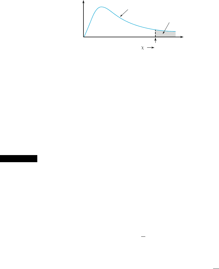
For example, moving down to tail area .085 and across to the 4 df column, we see that

the area to the right of 8.18 under the 4 df chi-squared curve is .085 (see Figure 13.2).

To capture this same upper-tail area under the 10 df curve, we must go out to

16.54. In the 2 df column, the top row shows that if the calculated value of the chi-

squared variable is smaller than 4.60, the captured tail area (the P-val ue) exceeds

.10. Similarly, the bottom row in this column indicates that if the calculated value

exceeds 13.81, the tail area is smaller than .001 (P-value < .001).

When the p

’s Are Functions of Other Parameters

Frequently the p

’s are hypothesized to depend o n a smaller number of parameters

, ... , y

(m < k). Then a specific hypothesis involving the y

’s yields specific

’s, which are then used in the w

test.

Example 13.2 In a well-known genetics article (“The Progeny in Generations F

to F

of a Cross

Between a Yellow-Wrinkled and a Green-Round Seeded Pea,” J. Genet.,1923:

255–331), the early statistician G. U. Yule analyzed data resulting from crossing

garden peas. The dominant alleles in the experiment were Y ¼ yellow color and

R ¼ round shape, resulting in the double dominant YR. Yule examined 269 four-

seed pods resulting from a dihybrid cross and counted the number of YR seeds in

each pod. Letting X denote the number of YR’s in a randomly selected pod, possible

X values are 0, 1, 2, 3, 4, which we identify with cells 1, 2, 3, 4, and 5 of a rectangular

table (so, for example, a pod with X ¼ 4 yields an observed count in cell 5).

The hypothesis that the Mendelian laws are operative and that genotypes of

individual seeds within a pod are independent of one another implies that X has a

binomial distribution with n ¼ 4 and y ¼

. We thus wish to test H

: p

¼ p

, ...,

¼ p

, where

¼ Pði  1YR

s among 4 seeds when H

is trueÞ

i  1



i1

ð1  yÞ

4ði1Þ

i ¼ 1; 2; 3; 4; 5; y ¼

Shaded area = .085

Chi-squared curve for 4 df

8.18

Calculated

Figure 13.2 A P-value for an upper-tailed chi-squared test

728

CHAPTER 13 Goodness-of-Fit Tests and Categorical Data Analysis

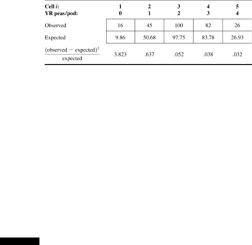
Yule’s data and the computations are in Table 13.3 with expected cell counts

¼ 269p

Thus w

¼ 3.823 + · · · + .032 ¼ 4.582. Since w

:01;k1

¼ w

:01;4

¼ 13:277,

is not rejected at level .01. Appendix Table A.10 shows that because

4.582 < 7.77, the P-value for the test exceeds .10. H

should not be rejected at

any reasonable significance level. ■

When the Underlying Distribution Is Continuous

We have so far assumed that the k categories are naturally defined in the context of

the experiment under consideration. The w

test can also be used to test whether a

sample comes from a specific underlying continuous distribution. Let X denote the

variable being sampled and suppose the hypothesized pdf of X is f

(x). As in the

construction of a frequency distribution in Chapter 1, subdivide the measurement

scale of X into k intervals [a

, a

), [a

, a

), ...,[a

k–1

, a

), where the interval [a

i–1,

)

includes the value a

i–1

but not a

The cell probabilities specified by H

are then

¼ Pða

i1

 X < a

Þ¼

i1

ðxÞdx

The cells should be chosen so that np

 5 for i ¼ 1, ... , k. Often they are

selected so that the np

’s are equal.

Example 13.3 To see whether the time of onset of labor among expectant mothers is uniformly

distributed throughout a 24 h day, we can divide a day into k periods, each of length

24/k. The null hypothesis states that f(x) is the uniform pdf on the interval [0, 24], so

that p

¼ 1/k. The article “The Hour of Birth” (Brit. J. Prevent. Social Med., 1953:

43–59) reports on 1186 onset times, which were categorized into k ¼ 24 1-hour

intervals beginning at midnight, resulting in cell counts of 52, 73, 89, 88, 68, 47, 58,

47, 48, 53, 47, 34, 21, 31, 40, 24, 37, 31, 47, 34, 36, 44, 78, and 59. Each expected

cell count is 1186  1/24 ¼ 49.42, and the resulting value of w

is 162.77. Since

:01;23

¼ 41:637, the computed value is highly significant, and the null hypothesis

is resoundingly rejected. Generally speaking, it appea rs that labor is much more

likely to commence very late at night than during normal waking hours.

■

For testing whether a sample comes from a specific normal distribution, the

fundamental parameters are y

¼ m and y

¼ s, and each p

will be a function of

these parameters.

Table 13.3 Observed and expected cell counts for Example 13.2

13.1 Goodness-of-Fit Tests When Category Probabilities Are Completely Speciﬁed 729

Example 13.4 The developers of a new standardized exam want it to satisfy the following criteria:

(1) actual time taken to complete the test is normally distributed, (2) m ¼ 100 min,

and (3) exactly 90% of all students will finish within a 2 h period. In the pilot testing

of the standardized test, 120 students are given the test, and their completion times

are recorded. For a chi-squared test of normally distributed completion time it is

decided that k ¼ 8 intervals should be used. The criteria imply that the 90th

percentile of the completion time distribution is m + 1.28s ¼ 2h¼ 120 min.

Since m ¼ 100, this implies that s ¼ 15.63.

The eight intervals that divide the standard normal scale into eight equally

likely segments are [0, .32), [.32, .675), [.675, 1.15), [1.15, 1), and their

four counterparts on the other side of 0. For m ¼ 100 and s ¼ 15.63, these

intervals become [100, 105), [105, 110.55), [110.55, 117.97), and [117.97, 1).

Thus p

¼ :125 ði ¼ 1; ...; 8Þ, from which each expected cell count is

¼ 120(.125) ¼ 15. The observed cell counts were 21, 17, 12, 16, 10, 15, 19,

and 10, resulting in a w

of 7.73. Since w

:10;7

¼ 12:017 and 7.73 is not  12.017,

there is no evidence for concluding that the criteria have not been met. ■

Exercises Section 13.1 (1–11)

1. What conclusion would be appropriate for an

upper-tailed chi-squared test in each of the follow-

ing situations?

a. a ¼ .05, df ¼ 4, w

¼ 12.25

b. a ¼ .01, df ¼ 3, w

¼ 8.54

c. a ¼ .10, df ¼ 2, w

¼ 4.36

d. a ¼ .01, k ¼ 6, w

¼ 10.20

2. Say as much as you can about the P-value for an

upper-tailed chi-squared test in each of the follow-

ing situations:

a. w

¼ 7.5, df ¼ 2

b. w

¼ 13.0, df ¼ 6

c. w

¼ 18.0, df ¼ 9

d. w

¼ 21.3, k ¼ 5

e. w

¼ 5.0, k ¼ 4

3. A statistics department at a large university main-

tains a tutoring center for students in its introduc-

tory service courses. The center has been staffed

with the expectation that 40% of its clients would

be from the business statistics course, 30% from

engineering statistics, 20% from the statistics

course for social science students, and the other

10% from the course for agriculture students.

A random sample of n ¼ 120 clients revealed

52, 38, 21, and 9 from the four courses. Does

this data suggest that the percentages on which

staffing was based are not correct? State and test

the relevant hypotheses using a ¼ .05.

4. It is hypothesized that when homing pigeons are

disoriented in a certain manner, they will exhibit

no preference for any direction of flight after

takeoff (so that the direction X should be uni-

formly distributed on the interval from 0



360



). To test this, 120 pigeons are disoriented,

let loose, and the direction of flight of each is

recorded; the resulting data follows. Use the chi-

squared test at level .10 to see whether the data

supports the hypothesis.

Direction 0– < 45



45– < 90



90– < 135



Frequency 12 16 17

Direction 135– < 180



180– < 225



225– < 270



Frequency 15 13 20

Direction 270– < 315



315– < 360



Frequency 17 10

5. An information retrieval system has ten storage

locations. Information has been stored with the

expectation that the long-run proportion of

requests for location i is given by the expression

¼ (5.5 – | i – 5.5| )/30. A sample of 200 retrieval

requests gave the following frequencies for loca-

tions 1–10, respectively: 4, 15, 23, 25, 38, 31, 32,

14, 10, and 8. Use a chi-squared test at significance

level .10 to decide whether the data is consistent

with the a priori proportions (use the P-value

approach).

6. Sorghum is an important cereal crop whose qual-

ity and appearance could be affected by the pres-

ence of pigments in the pericarp (the walls of the

730 CHAPTER 13 Goodness-of-Fit Tests and Categorical Data Analysis

plant ovary). The article “A Genetic and Biochem-

ical Study on Pericarp Pigments in a Cross

Between Two Cultivars of Grain Sorghum, Sor-

ghum Bicolor” (Heredity, 1976: 413–416) reports

on an experiment that involved an initial cross

between CK60 sorghum (an American variety

with white seeds) and Abu Taima (an Ethiopian

variety with yellow seeds) to produce plants with

red seeds and then a self-cross of the red-seeded

plants. According to genetic theory, this F

cross

should produce plants with red, yellow, or white

seeds in the ratio 9:3:4. The data from

the experiment follows; does the data confirm or

contradict the genetic theory? Test at level .05

using the P-value approach.

Seed Color Red Yellow White

Observed Frequency 195 73 100

7. Criminologists have long debated whether there is

a relationship between weather conditions and the

incidence of violent crime. The author of the arti-

cle “Is There a Season for Homicide?” (Criminol-

ogy, 1988: 287–296) classified 1361 homicides

according to season, resulting in the accompany-

ing data. Test the null hypothesis of equal propor-

tions using a ¼ .01 by using the chi-squared table

to say as much as possible about the P-value.

Winter Spring Summer Fall

328 334 372 327

8. The article “Psychiatric and Alcoholic Admissions

Do Not Occur Disproportionately Close to

Patients’ Birthdays” (Psych. Rep., 1992: 944–946)

focuses on the existence of any relationship

between date of patient admission for treatment of

alcoholism and patient’s birthday. Assuming a 365-

day year (i.e., excluding leap year), in the absence

of any relation, a patient’s admission date is equally

likely to be any one of the 365 possible days. The

investigators established four different admission

categories: (1) within 7 days of birthday, (2)

between 8 and 30 days, inclusive, from the birth-

day, (3) between 31 and 90 days, inclusive, from

the birthday, and (4) more than 90 days from the

birthday. A sample of 200 patients gave observed

frequencies of 11, 24, 69, and 96 for categories 1, 2,

3, and 4, respectively. State and test the relevant

hypotheses using a significance level of .01.

9. The response time of a computer system to a

request for a certain type of information is

hypothesized to have an exponential distribution

with parameter l ¼ 1 [so if X ¼ response time,

the pdf of X under H

is f

(x) ¼ e

–x

for x  0].

a. If you had observed X

, X

, ..., X

and wanted

to use the chi-squared test with five class inter-

vals having equal probability under H

, what

would be the resulting class intervals?

b. Carry out the chi-squared test using the follow-

ing data resulting from a random sample of 40

response times:

.10 .99 1.14 1.26 3.24 .12 .26 .80

.79 1.16 1.76 .41 .59 .27 2.22 .66

.71 2.21 .68 .43 .11 .46 .69 .38

.91 .55 .81 2.51 2.77 .16 1.11 .02

2.13 .19 1.21 1.13 2.93 2.14 .34 .44

10. a. Show that another expression for the chi-

squared statistic is

i¼1

 n

Why is it more efficient to compute w

using

this formula?

b. When the null hypothesis is H

: p

¼ p

¼ 

¼ p

¼ 1/k (i.e., p

¼ 1/k for all i), how does

the formula of part (a) simplify? Use the sim-

plified expression to calculate w

for the

pigeon/direction data in Exercise 4.

11. a. Having obtained a random sample from a

population, you wish to use a chi-squared

test to decide whether the population dis-

tribution is standard normal. If you base the

test on six class intervals having equal pro-

bability under H

, what should the class

intervals be?

b. If you wish to use a chi-squared test to test H

the population distribution is normal with

m ¼ .5, s ¼ .002 and the test is to be based

on six equiprobable (under H

) class intervals,

what should these intervals be?

c. Use the chi-squared test with the intervals of

part (b) to decide, based on the following 45

bolt diameters, whether bolt diameter is a nor-

mally distributed variable with m ¼ .5 in., s

¼ .002 in.

.4974 .4976 .4991 .5014 .5008 .4993

.4994 .5010 .4997 .4993 .5013 .5000

.5017 .4984 .4967 .5028 .4975 .5013

.4972 .5047 .5069 .4977 .4961 .4987

.4990 .4974 .5008 .5000 .4967 .4977

.4992 .5007 .4975 .4998 .5000 .5008

.5021 .4959 .5015 .5012 .5056 .4991

.5006 .4987 .4968

13.1 Goodness-of-Fit Tests When Category Probabilities Are Completely Speciﬁed 731

13.2

Goodness-of-Fit Tests for Composite

Hypotheses

In the previous section, we presented a goodness-of-fit test based on a w

statistic

for deciding between H

: p

¼ p

, ..., p

¼ p

and the alternative H

stating that

is not true. The null hypothesis was a simpl e hypothesis in the sense that each p

was a specified number, so that the expected cell counts when H

was true were

uniquely determined numbers.

In many situations, there are k naturally occurring categories, but H

states

only that the p

’s are functions of other parameters y

, ... , y

without specifying

the values of these y’s. For example, a population may be in equilibrium with

respect to proportions of the three genotypes AA, Aa, and aa. With p

, p

, and p

denoting these proportions (probabilities), one may wish to test

: p

¼ y

; p

¼ 2yð1  yÞ; p

¼ð1  y Þ

ð13:1Þ

where y represents the proportion of gene A in the population. This hypothesis is

composite because knowing that H

is true does not uniquely determine the cell

probabilities and expected cell counts but only their general form. To carry out a

test, the unknown y

’s must first be estimated.

Similarly, we may be interested in testing to see whether a sample came from

a particular family of distributions without specifying any particular member of the

family. To use the w

test to see whether the distri bution is Poisson, for example, the

parameter l must be estimated. In addition, because there are actually an infinite

number of possible values of a Poisson variable, these valu es must be grouped so

that there are a finite number of cells. If H

states that the underlying distribution

is normal, use of a w

test must be preceded by a choice of cells and estimation of

m and s.

When Parameters Are Estimated

As before, k will denote the number of categories or cells and p

will denote the

probability of an observation falling in the ith cell. The null hypothesis now states

that each p

is a function of a small number of parameters y

, ... , y

with the y

’s

otherwise unspecified:

: p

¼ p

ðuÞ; ...; p

¼ p

ðuÞ where u ¼ðy

; ...; y

: the hypothesis H

is not true

ð13:2Þ

For example, for H

of (13.1), m ¼ 1 (there is only one y), p

(y) ¼ y

, p

(y) ¼

2y(1 – y), and p

(y) ¼ (1 – y)

In the case k ¼ 2, there is really only a single rv, N

(since N

¼ n),

which has a binomial distribution. The joint probability that N

¼ n

and N

¼ n

is then

PðN

¼ n

; N

¼ n

Þ¼



/ p

732 CHAPTER 13 Goodness-of-Fit Tests and Categorical Data Analysis

where p

¼ 1 and n

¼ n. For general k, the joint distribution of N

, ...,

is the multinomial distribution (Section 5.1)with

PðN

¼ n

; :::; N

¼ n

Þ/p

p

ð13:3Þ

When H

is true, (13.3) becomes

PðN

¼ n

; :::; N

¼ n

Þ/½p

ðuÞ





½p

ðuÞ

ð13:4Þ

To apply a chi-squared test, y ¼ (y

, ... , y

) must be estimated.

METHOD OF

ESTIMATION

Let n

, n

, ..., n

denote the observed values of N

, ..., N

. Then

; ...;

are those values of the y

’s that maximize (13.4), that is, the maximum

likelihood estimators (Section 7.2).

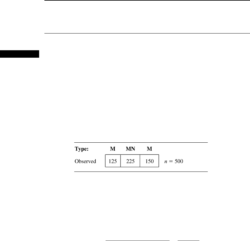
Example 13.5 In humans there is a blood group, the MN group, that is composed of individuals

having one of the three blood types M, MN, and N. Type is determined by two alleles,

and there is no dominance, so the three possible genotypes give rise to three pheno-

types. A population consisting of individuals in the MN group is in equilibrium if

PðMÞ¼p

¼ y

PðMNÞ¼p

¼ 2yð1  yÞ

PðNÞ¼p

¼ð1  yÞ

for some y. Suppose a sample from such a population yielded the results shown in

Table 13.4.

Then

½p

ðyÞ

½p

ðyÞ

½p

ðyÞ

¼½y



½2yð1  yÞ

½ð1  yÞ



¼ 2

 y

þn

ð1  yÞ

þ2n

Maximizing this with respect to y (or, equivalently, max imizing the natural loga-

rithm of this quantity, which is easier to differentiate) yields

y ¼

þ n

½ð2n

þ n

Þþðn

þ 2n

Þ

þ n

With n

¼ 125 and n

¼ 225,

y ¼ 475=1000 ¼ :475. ■

Once u ¼ (y

, ..., y

) has been estimated by

u ¼ð

; ...;

Þ, the estimated

expected cell counts are the np

uÞ’s. These are now used in place of the np

’s of

Section 13.1 to specify a w

statistic.

Table 13.4 Observed counts for Example 13.5

13.2 Goodness-of-Fit Tests for Composite Hypotheses 733

THEOREM

Under general “regularity” conditions on y

, ..., y

and the p

(u)’s, if y

, ...,

are estimated by the method of maximum likelihood as described previ-

ously and n is large,

all cells

ðobserved  estimated expectedÞ

expected

i¼1

½N

 np

uÞ

uÞ

has approximately a chi-squared distribution with k –1–m df when H

(13.2) is true. An approximately level a test of H

versus H

is then to reject

if w

 w

a;k1m

. In practice, the test can be used if np

uÞ5 for every i.

Notice that the number of degrees of freedom is reduced by the number of y

’s

estimated.

Example 13.6

(Example 13.5

continued)

With

y ¼ :475 and n ¼ 500, the estimated expected cell counts are

yÞ¼500ð

yÞ

¼112:81, np

yÞ¼ 500ðÞ2ðÞ:475ðÞð1:475Þ¼ 249:38, and

yÞ¼500 112:81 249:38 ¼137:81. Then

ð125  112:81Þ

112:81

ð225  249:38Þ

249:38

ð150  137:81Þ

137:81

¼ 4:78

Since w

:05;k1m

¼ w

:05;311

¼ w

:05;1

¼ 3:843 and 4.78  3.843, H

is rejected.

Appendix Table A.10 shows that P-value  .029.

■

Example 13.7 Consider a series of games between two teams, I and II, that terminates as soon as

one team has won four games (with no possibility of a tie). A simple proba bility

model for such a series assumes that outcomes of successive games are independent

and that the probability of team I winning any particular game is a constant y.We

arbitrarily designate I the better team, so that y  .5. Any particular series can then

terminate after 4, 5, 6, or 7 games. Let p

(y), p

(y) denote the

probability of termination in 4, 5, 6, and 7 games, respectively. Then

ðyÞ¼PðI wins in 4 gamesÞþPðII wins in 4 gamesÞ

¼ y

þ 1  yðÞ

ðyÞ¼PðI wins 3 of the first 4 and the fifthÞ

þ PðI loses 3 of the first 4 and the fifthÞ



ð1  yÞy þ



yð1  yÞ

ð1  yÞ

¼ 4y 1  yðÞy

þ 1  yðÞ

ðyÞ¼10y

ð1  yÞ

½y

þð1  yÞ



ðyÞ¼20y

ð1  yÞ

The article “Seven-Game Series in Sports” by Groeneveld and Meeden

(Math. Mag., 1975: 187–192) tested the fit of this model to results of National

734 CHAPTER 13 Goodness-of-Fit Tests and Categorical Data Analysis

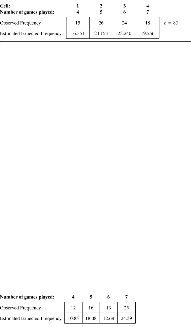
Hockey League playoffs during the period 1943–1967 (when league membership

was stable). The data appears in Table 13.5 .

The estimated expected cell counts are 83p

yÞ, where

y is the value of y that

maximizes

þ 1  yðÞ

 4y 1  yðÞy

þ 1  yðÞ

hino

 10y

1  yðÞ

þ 1  yðÞ

hino

 20y

1  yðÞ

ð13:5Þ

Standard calculus methods fail to yield a nice formula for the maximizing value

so it must be computed using numerical methods. The result is

y ¼ :654, from which

yÞ and the estimated expected cell counts are computed. The computed value of

is .360, and (since k –1–m ¼ 4–1–1¼ 2) w

:10;2

¼ 4:605. There is thus no

reason to reject the simple model as applied to NHL playoff series.

The cited article also considered World Series data for the period 1903–1973.

For the simple model, w

¼ 5.97, so the model does not seem appropriate. The

suggested reason for this is that for the simple model

Pðseries lasts six games jseries lasts at least six games Þ:5 ð13:6Þ

whereas of the 38 series that actually lasted at least six games, only 13 lasted

exactly six. The following alternative model is then introduced:

ðy

; y

Þ¼y

þð1  y

ðy

; y

Þ¼4y

ð1  y

Þ½y

þð1  y



ðy

; y

Þ¼10y

1  y

ðÞ

ðy

Þ¼10y

ð1  y

The first two p

’s are identical to the simple model, whereas y

is the conditional

probability of (13.6) (which can now be any number between zero and one).

The values of

and

that maximize the expression analogous to expression

(13.5) are determined numerically as

¼ :614,

¼ :342. A summary appears in

Table 13.6,andw

¼ .384. Two parameters are estimated, so df ¼ k–1–m ¼ 1

with w

:10;1

¼ 2:706, indicating a good fit of the data to this new model.

Table 13.6 Observed and expected counts for the more complex model

■

Table 13.5 Observed and expected counts for the simple model

13.2 Goodness-of-Fit Tests for Composite Hypotheses 735

One of the regularity conditions on the y

’s in the theorem is that they be

functionally independent of one another. That is, no sing le y

can be determ ined

from the values of other y

’s, so that m is the number of functionally independent

parameters estimat ed. A general rule of thumb for degrees of freedom in a chi-

squared test is the following.

df ¼

number of freely

determined cell counts





number of independent

parameters estimated



This rule will be used in connection with several different chi-squared tests in the

next section.

Goodness of Fit for Discrete Distributions

Many experiments involve observing a random sample X

, X

, ..., X

from some

discrete distribution. One may then wish to investigate whether the underlying

distribution is a member of a particular family, such as the Poisson or negative

binomial family. In the case of both a Poisson and a negative binomial distribution,

the set of possible values is infinite, so the values must be grouped into k subsets

before a chi-squared test can be used. Th e groupings should be done so that the

expected frequency in each cell (group) is at least 5. The last cell will then

correspond to X values of c, c +1,c +2,... for some value c.

This grouping can considerably complicate the computation of the

’s and

estimated expected cell counts. This is because the theorem requires that the

’s be

obtained from the cell counts N

, ..., N

rather than the sample values X

, ..., X

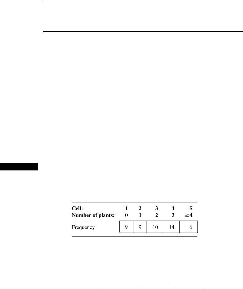
Example 13.8 Table 13.7 presents count data on the number of Larrea divaricata plants found in

each of 48 sampling quadrats, as reported in the article “Some Sampling Character-

istics of Plants and Arthropods of the Arizona Desert” (Ecology, 1962: 567–571).

The author fit a Poisson distribution to the data. Let l denote the Po isson

parameter and suppose for the moment that the six counts in cell 5 were actually 4,

4, 5, 5, 6, 6. Then denoting sample values by x

, ..., x

, nine of the x

’s were 0, nine

were 1, and so on. The likelihood of the observed sample is

l



l

48l

!x

48l

101

!x

The value of l for which this is maximized is

l ¼ x

=n ¼ 101=48 ¼ 2:10 (the value

reported in the article).

Table 13.7 Observed counts for Example 13.8

736 CHAPTER 13 Goodness-of-Fit Tests and Categorical Data Analysis

However, the

l require d for w

is obtained by maximizing Expression (13.4)

rather than the likelihood of the full sample. The cell probabilities are

ðlÞ¼

l

i1

ði  1Þ!

i ¼ 1; 2; 3; 4

ðlÞ¼1 

i¼0

l

so the right-hand side of (13.4) becomes

l



l



l



l



1 

i¼0

l

ð13:7Þ

There is no nice formula for

l, the maximizing value of l in this latter expression,

so it must be obtained numerically. ■

Because the parameter estimates are usually much more difficult to compute

from the grouped data than from the full sample, they are often computed usin g this

latter method. When these “full” estimators are used in the chi-squared statistic, the

distribution of the statistic is altered and a level a test is no longer specified by the

critical value w

a;k1m

THEOREM

Let

; ...;

be the maximum likelihood estimators of y

, ..., y

based on

the full sample X

, ..., X

, and let w

denote the statistic based on these

estimators. Then the critical value c

that specifies a level a upper-tailed test

satisfies

a;k1m

 c

 w

a;k1

ð13:8Þ

The test procedure implied by this theorem is the following:

If w

 w

a;k1

; reject H

If w

 w

a;k1m

; do not reject H

: ð13:9Þ

If w

a;k1m

< w

a;k1

; withhold judgment:

13.2 Goodness-of-Fit Tests for Composite Hypotheses 737