Dinc Ibrahim. Refrigeration systems and applications 2th edition

Подождите немного. Документ загружается.

Advanced Refrigeration Cycles and Systems 221

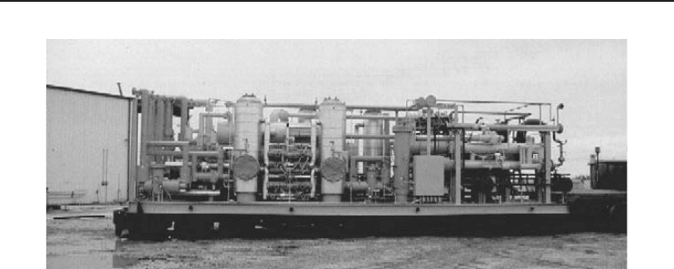
Figure 5.2 A cascade refrigeration system utilizing CO

as low-pressure stage refrigerant and ammonia as

the high-pressure stage refrigerant (operating at about −50

◦

C), skid for a 100 ton/day CO

liquefaction plant

(Courtesy of Salof Refrigeration Co., Inc.).

Conventional single compressor, mechanical refrigeration system condensing units are capa-

ble of achieving temperatures of about −40

◦

C. If lower temperatures are required then cascade

refrigeration systems must be used. A two-stage cascade system uses two refrigeration systems

connected in series to achieve temperatures of around −85

◦

C. There are single compressor sys-

tems that can achieve temperatures colder than −100

◦

C but they are not widely used. These systems

are sometimes referred to as autocascading systems. The main disadvantage of such systems is

that it requires the use of a proprietary blend of refrigerant. This characteristic results in three

service-related problems:

• A leak in the system can easily cause the loss of only some of the refrigerant making up the

blend (since the refrigerant blend is made up of different types of refrigerant with different

boiling points), resulting in an imbalance in the ratio of the remaining refrigerants. To return the

system to proper operation, all of the remaining refrigerant must be replaced with a new and

potentially costly charge to ensure a proper blend ratio.

• The blend is proprietary and may not be readily available from the traditional refrigerant supply

sources and therefore may be hard to obtain and costly.

• These types of cascade systems are not widely used; it is hard to ﬁnd well-qualiﬁed ﬁeld service

staff who are familiar with repair and maintenance procedures.

Of course, these and other issues can cause undesirable expense and downtime.

5.3.1 Two-Stage Cascade Systems

A two-stage cascade system employs two vapor-compression units working separately with different

refrigerants and interconnected in such a way that the evaporator of one system is used to serve as

condenser to a lower temperature system (i.e., the evaporator from the ﬁrst unit cools the condenser

of the second unit). In practice, an alternative arrangement utilizes a common condenser with a

booster circuit to provide two separate evaporator temperatures.

In fact, the cascade arrangement allows one of the units to be operated at a lower temperature

and pressure than would otherwise be possible with the same type and size of single-stage system.

It also allows two different refrigerants to be used, and it can produce temperatures below −150

◦

Figure 5.3 shows a two-stage cascade refrigeration system, where condenser B of system 1 is being

cooled by evaporator C of system 2. This arrangement enables reaching ultralow temperatures in

evaporator A of the system.

222 Refrigeration Systems and Applications

Low-stage compression

Oil separator Oil separato

High-stage compression

Evaporator

Condenser

evaporator

Heat

exchanger

Bypass valve

TEV

Thermal expansion value

Figure 5.3 A practical two-stage cascade refrigeration system.

(

)(

)

Expansion

valve

Expansion

valve

Compressor

Heat exchanger

Evaporator

Condenser

Heat

Decrease in

compressor

work

Increase in refrigeration capacity

Log P (kPa)

h (kJ/kg)

Evaporator

Condenser

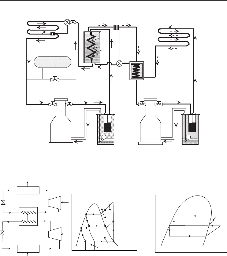
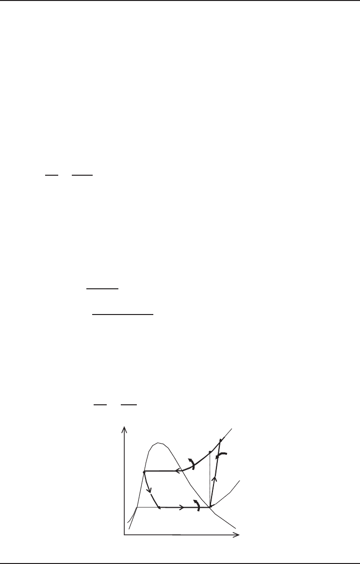
Figure 5.4 (a) Schematic of a two-stage (binary) cascade refrigeration system, (b) its T–s diagram, and (c) its

log P–h diagram. [Adapted from Cengel and Boles (2008).]

For a schematic system shown in Figure 5.4, the condenser of system I, called the ﬁrst or high-

pressure stage, is usually fan cooled by the ambient air. In some cases a water supply may be used,

but air cooling is much more common. The evaporator of system I is used to cool the condenser of

system II called the second or low-pressure stage. The unit that makes up the evaporator of system I

and the condenser of system II is often referred to as the inter-stage or cascade condenser. As stated

earlier, cascade systems generally use two different refrigerants (i.e., one in each stage). One type

is used for the low stage and a different one for the high stage. The reason why two refrigeration

systems are used is that a single system cannot economically achieve the high compression ratios

Advanced Refrigeration Cycles and Systems 223

necessary to obtain the proper evaporating and condensing temperatures. It is clear from the T −s

diagram of the two-stage cascade refrigeration system, as shown in Figure 5.4, that the compressor

work decreases and the amount of refrigeration load (capacity) in the evaporator increases as a

result of cascading (Cengel and Boles, 2008). Therefore, cascading improves the COP.

Example 5.1

Consider a two-stage cascade refrigeration system operating between the pressure limits of 1.6 MPa

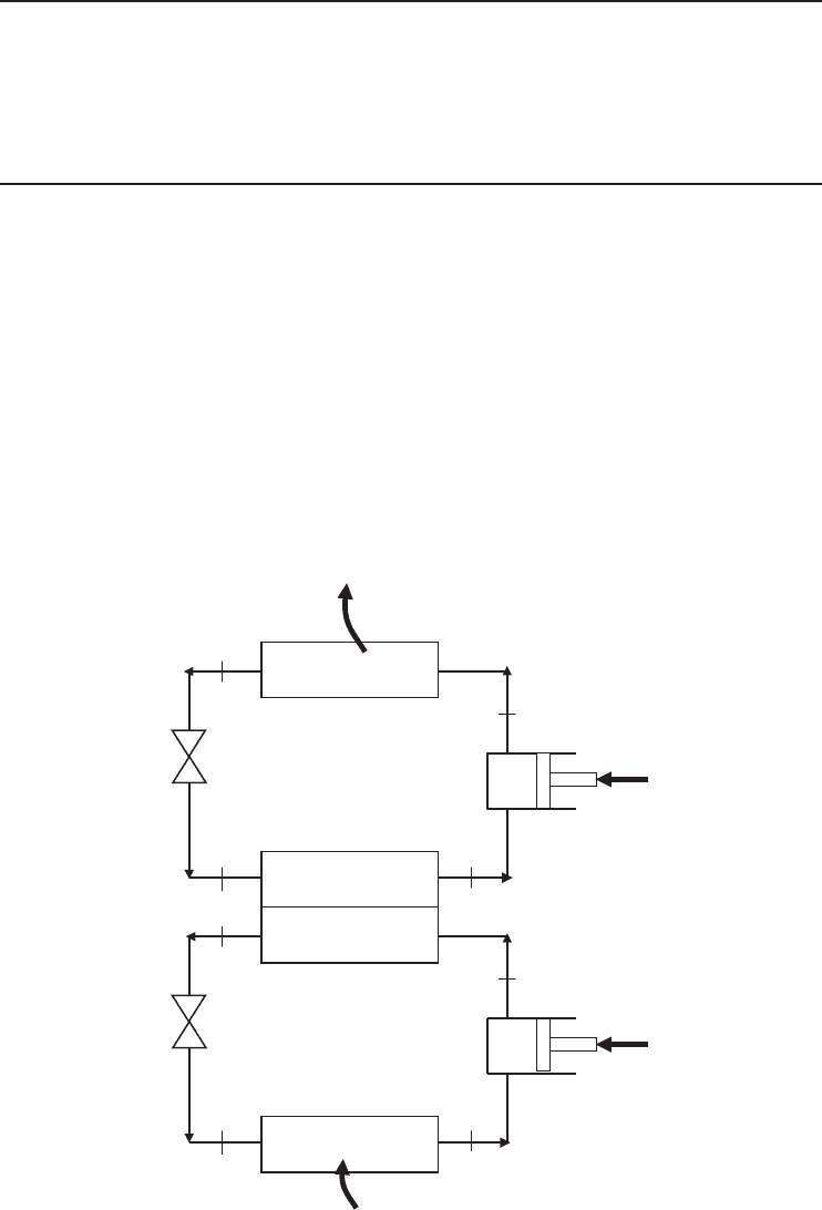
and 180 kPa with refrigerant-134a as the working ﬂuid (Figure 5.5). Heat rejection from the lower

cycle to the upper cycle takes place in an adiabatic counter-ﬂow heat exchanger where the pressure

in the upper and lower cycles are 0.4 and 0.5 MPa, respectively. In both cycles, the refrigerant

is a saturated liquid at the condenser exit and a saturated vapor at the compressor inlet, and the

isentropic efﬁciency of the compressor is 85%. If the mass ﬂow rate of the refrigerant through the

lower cycle is 0.07 kg/s, (a) draw the temperature–entropy diagram of the cycle indicating pressures;

determine (b) the mass ﬂow rate of the refrigerant through the upper cycle, (c) the rate of heat

removal from the refrigerated space, and (d) the COP of this refrigerator; and (e) determine the

rate of heat removal and the COP if this refrigerator operated on a single-stage cycle between the

same pressure limits with the same compressor efﬁciency. Also, take the mass ﬂow rate of R-134a

through the cycle to be 0.07 kg/s.

Condenser

Evaporator

Compressor

Condenser

Evaporator

Compressor

Figure 5.5 Schematic of two-stage cascade refrigeration system considered in Example 5.1.

224 Refrigeration Systems and Applications

Solution

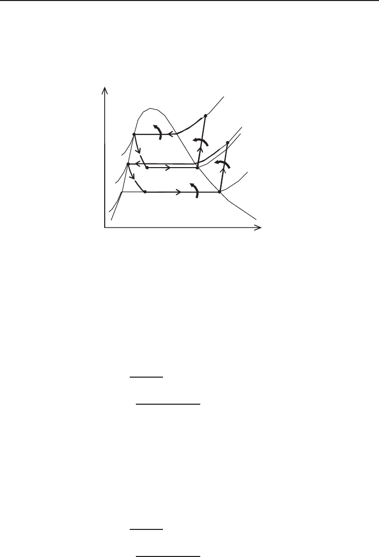
(a) Noting that compression processes are not isentropic, the temperature–entropy diagram of the

cycle can be drawn as shown in Figure 5.6.

0.18 MPa

0.5 MPa

0.4 MPa

1.6 MPa

0.5 MPa

Figure 5.6 T–s diagram of the system considered in Example 5.1.

(b) The properties are to be obtained from the refrigerant-134a tables (Tables B.3 through B.5):

= h

g@180 kPa

= 242.86 kJ/kg

= s

g@180 kPa

= 0.9397 kJ/kg · K

= 500 kPa

= s



= 263.86 kJ/kg

− h

0.85 =

263.86 − 242.86

− 242.86

−→ h

= 267.57 kJ/kg

= h

f @500 kPa

= 73.33 kJ/kg

= h

= 73.33 kJ/kg

= h

g@400 kPa

= 255.55 kJ/kg

= s

g@400 kPa

= 0.9269 kJ/kg · K

= 1600 kPa

= s



= 284.22 kJ/kg

− h

0.85 =

284.22 − 255.55

− 255.55

−→ h

= 289.28 kJ/kg

= h

f @1600 kPa

= 135.93 kJ/kg

= h

= 135.93 kJ/kg

Advanced Refrigeration Cycles and Systems 225

The mass ﬂow rate of the refrigerant through the upper cycle is determined from an energy

balance on the heat exchanger.

˙m

− h

) =˙m

− h

)

˙m

(255.55 − 135.93) kJ/kg = (0.07 kg/s)(267.57 − 73.33) kJ/kg −→ ˙m

= 0.1137 kg/s

=˙m

− h

) = (0.07 kg/s)(242.86 − 73.33) kJ/kg = 11.87 kW

(d) The power input and the COP are

W =˙m

− h

) +˙m

− h

)

= (0.1137 kg/s)(289.28−255.55) kJ/kg + (0.07 kg/s)(267.57−242.86) kJ/kg = 5.56 kW

COP =

11.87

5.56

= 2.13

(e) If this refrigerator operated on a single-stage cycle (Figure 5.7) between the same pressure

limits, we would have

= h

g@180 kPa

= 242.86 kJ/kg

= s

g@180 kPa

= 0.9397 kJ/kg · K

= 1600 kPa

= s



= 288.52 kJ/kg

− h

0.85 =

288.52 − 242.86

− 242.86

−→ h

= 296.58 kJ/kg

= h

f @1600 kPa

= 135.93 kJ/kg

= h

= 135.93 kJ/kg

=˙m(h

− h

) = (0.07 kg/s)(242.86 − 135.93) kJ/kg = 7. 49 kW

W =˙m(h

− h

) = (0.07 kg/s)(296.58 − 242.86) kJ/kg = 3.76 kW

COP =

7.49

3.76

= 1.99

0.18 MPa

1.6 MPa

Figure 5.7 T–s diagram of the single-stage cycle considered in part (d) of Example 5.1.

226 Refrigeration Systems and Applications

Cooling

water

or air

Propane

Natural gas from pipeline

Q′

Ethane

Gas at

−37 °C

Q′

Methane

Liquefied gas at

−82 °C

Liquefied storage at

−157 °C

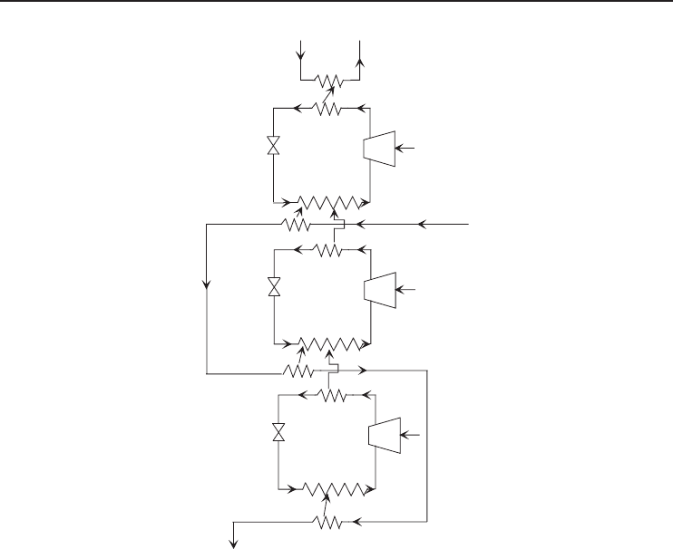
Figure 5.8 A three-stage (ternary) cascade vapor-compression refrigeration system.

5.3.2 Three-Stage (Ternary) Cascade Refrigeration Systems

Cascade refrigeration cycles are commonly used in the liquefaction of natural gas, which consists

basically of hydrocarbons of the parafﬁn series, of which methane has the lowest boiling point at

atmospheric pressure. Refrigeration down to that temperature can be provided by a ternary cascade

refrigeration cycle using propane, ethane, and methane, whose boiling points at standard atmospheric

pressure are 231.1, 184.5, and 111.7 K, respectively (Haywood, 1980). A simpliﬁed basic diagram

for such a cascade cycle is shown in Figure 5.8. In the operation, the compressed methane vapor is

ﬁrst cooled by heat exchange with the propane in the propane evaporator before being condensed by

heat exchange with the ethane in the ethane evaporator, thus reducing the degree of irreversibility

involved in the cooling and condensation of the methane. Also, because of the high temperature

after compression, the gas leaving each compressor passes ﬁrst through a water-cooled intercooler.

In a large-scale plant of this type, the compressors become rotary turbomachines instead of the

reciprocating types.

5.4 Liquefaction of Gases

Cryogenics is associated with low temperatures, usually deﬁned to be below −100

◦

C (173 K).

The general scope of cryogenic engineering is the design, development, and improvement of

Advanced Refrigeration Cycles and Systems 227

low-temperature systems and components. The applications of cryogenic engineering include

liquefaction of gases, separation of gases, high-ﬁeld magnets, and sophisticated electronic devices

that use the superconductivity property of materials at low temperatures, space simulation,

food freezing, medical procedures such as cryogenic surgery, and various chemical processes

(ASHRAE, 2006; Dincer, 2003).

The liquefaction of gases has always been an important area of refrigeration since many important

scientiﬁc and engineering processes at cryogenic temperatures depend on liqueﬁed gases. Some

examples of such processes are the separation of oxygen and nitrogen from air, preparation of

liquid propellants for rockets, study of material properties at low temperatures, and study of some

exciting phenomena such as superconductivity. At temperatures above the critical-point value, a

substance exists in the gas phase only. The critical temperatures of helium, hydrogen, and nitrogen

(three commonly used liqueﬁed gases) are −268, −240, and −147

◦

C, respectively (Cengel and

Boles, 2008). Therefore, none of these substances will exist in liquid form at atmospheric conditions.

Furthermore, low temperatures of this magnitude cannot be obtained with ordinary refrigeration

techniques.

The general principles of various gas liquefaction cycles, including the Linde–Hampson cycle,

and their general thermodynamic analyses are presented elsewhere, for example, Timmerhaus and

Flynn (1989), Barron (1985), and Walker (1983).

Here we present the methodology for the ﬁrst- and second-law-based performance analyses of the

simple Linde–Hampson cycle, and investigate the effects of gas inlet and liquefaction temperatures

on various cycle performance parameters.

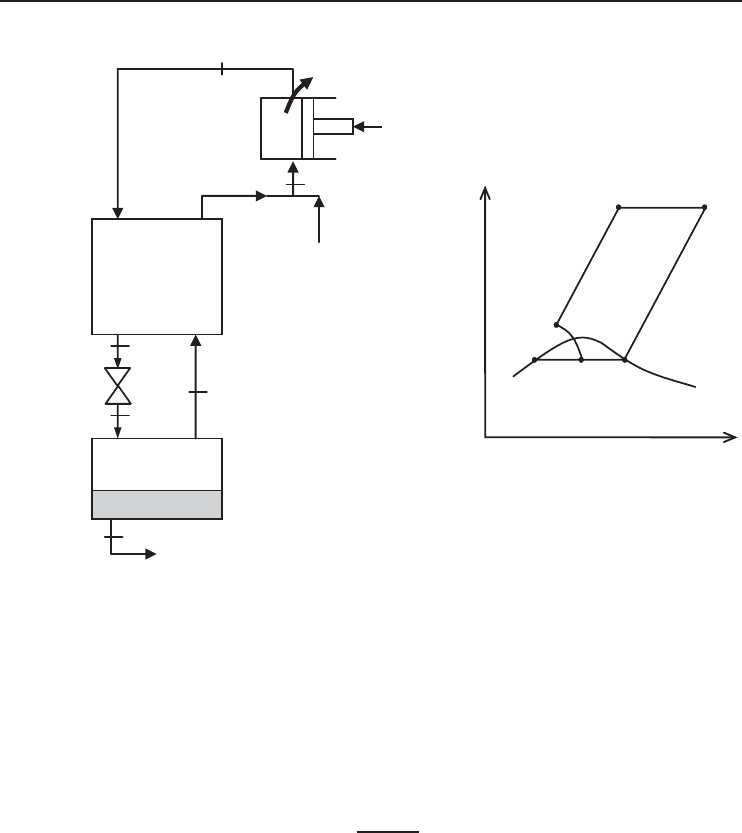
5.4.1 Linde–Hampson Cycle

Several cycles, some complex and others simple, are used successfully for the liquefaction of gases.

Here, we consider the simple Linde–Hampson cycle, which is shown schematically and on a T −s

diagram in Figure 5.9, in order to describe energy and exergy analyses of liquefaction cycles.

See Kanoglu et al. (2008) for details of the analysis in this section. Makeup gas is mixed with the

uncondensed portion of the gas from the previous cycle, and the mixture at state 1 is compressed by

an isothermal compressor to state 2. The temperature is kept constant by rejecting compression heat

to a coolant. The high-pressure gas is further cooled in a regenerative counter-ﬂow heat exchanger

by the uncondensed portion of gas from the previous cycle to state 3, and is then throttled to

state 4, where it is a saturated liquid–vapor mixture. The vapour (state 5) is routed through the heat

exchanger and the liquid (state 6) is collected as the desired product, to cool the high-pressure gas

approaching the throttling valve. Finally, the gas is mixed with fresh makeup gas, and the cycle

is repeated.

The refrigeration effect for this cycle can be deﬁned as the heat removed from the makeup gas

in order to turn it into a liquid at state 6. Assuming ideal operation for the heat exchanger (i.e., the

gas leaving the heat exchanger and the makeup gas are at the same state as state 1, which is the

compressor inlet state; this is also the dead state: T

= T

), the refrigeration effect per unit mass

of the liqueﬁed gas is given by

= h

− h

= h

− h

(per unit mass of liquefaction) (5.1)

where h

is the enthalpy of saturated liquid that is withdrawn. From an energy balance on the

cycle, the refrigeration effect per unit mass of the gas in the cycle prior to liquefaction may be

expressed as

= h

− h

(per unit mass of gas in the cycle) (5.2)

228 Refrigeration Systems and Applications

Compressor

Expansion

valve

Liquid

removed

(a) (b)

Heat

exchanger

Makeup gas

Figure 5.9 (a) Schematic and (b) temperature–entropy diagram for a simple Linde–Hampson liquefaction

cycle (Kanoglu et al., 2008).

Maximum liquefaction occurs when the difference between h

and h

(i.e., the refrigeration

effect) is maximized. The ratio of Equations 5.2 and 5.1 is the fraction of the gas in the cycle that

is liqueﬁed. That is,

y =

− h

(5.3)

An energy balance on the heat exchanger gives

− h

= x(h

− h

) (5.4)

where x is the quality of the mixture at state 4. The fraction of the gas that is liqueﬁed may also

be determined from

y = 1 − x (5.5)

An energy balance on the compressor gives the work of compression per unit mass of the gas

in the cycle as

actual

= h

− h

− T

− s

) (per unit mass of gas in the cycle) (5.6)

Advanced Refrigeration Cycles and Systems 229

Note that T

= T

. The last term in this equation is the isothermal heat rejection from the gas as

it is compressed. Considering that the gas generally behaves as an ideal gas during this isothermal

compression process, the compression work may also be determined from

actual

= RT





(5.7)

The COP of this cycle is given by

COP

actual

− h

− T

− s

)

(5.8)

In liquefaction cycles, a performance parameter used is the work consumed in the cycle for the

liquefaction of a unit mass of the gas. This is expressed as

actual

− h

− T

− s

)

(per unit mass of liquefaction) (5.9)

As the liquefaction temperature decreases work consumption increases. Noting that different

gases have different thermophysical properties and require different liquefaction temperatures, this

work parameter should not be used to compare work consumptions for the liquefaction of different

gases. A reasonable use is to compare different cycles used for the liquefaction of the same gas.

An important object of exergy analysis for systems that consume work such as liquefaction of

gases is ﬁnding the minimum work required for a certain desired result and comparing it to the

actual work consumption. The ratio of these two quantities is often considered the exergy efﬁciency

of such a liquefaction process (Kanoglu, 2002). Engineers are interested in comparing the actual

work used to obtain a unit mass of liqueﬁed gas to the minimum work required to obtain the

same output. Such a comparison may be performed using the second law of thermodynamics. For

instance, the minimum work input requirement (reversible work) and the actual work for a given

set of processes may be related to each other by

actual

= w

rev

+ T

gen

= w

rev

+ ex

dest

(5.10)

where T

is the environment temperature, s

gen

is the speciﬁc entropy generation, and ex

dest

is the

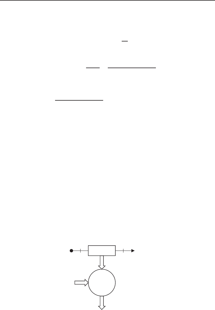
speciﬁc exergy destruction during the processes. The reversible work for the simple Linde–Hampson

cycle shown in Figure 5.10 may be expressed by the stream exergy difference of states 1 and 6 as

rev

= ex

− ex

= h

− h

− T

− s

) (5.11)

Carnot

refrigerator

Gas

Liquefied

gas

rev

Figure 5.10 A Carnot refrigerator that uses a minimum amount of work for a liquefaction process.

230 Refrigeration Systems and Applications

where state 1 has the properties of the makeup gas, which is usually the dead state. As this equation

clearly shows, the minimum work required for liquefaction depends only on the properties of the

incoming and outgoing gas being liqueﬁed and the ambient temperature T

. An exergy efﬁciency

may be deﬁned as the reversible work input divided by the actual work input, both per unit mass

of the liquefaction:

rev

actual

− h

− T

− s

)

(1/y)

[

− h

− T

− s

)

]

(5.12)

The exergy efﬁciency may also be deﬁned using actual and reversible COPs of the system as

COP

actual

COP

rev

(5.13)

where the reversible COP is given by

COP

rev

− h

− T

− s

)

(5.14)

The minimum work input for the liquefaction process is simply the work input required for the

operation of a Carnot refrigerator for a given heat removal, which can be expressed as

rev



δq



1 −



(5.15)

where δq is the differential heat transfer and T is the instantaneous temperature at the boundary

where the heat transfer takes place. Note that T is smaller than T

for the liquefaction process, and

to get a positive work input we have to take the sign of heat transfer to be negative since it is a heat

output. The evaluation of Equation 5.15 requires knowledge of the functional relationship between

the heat transfer δq and the boundary temperature T , which is usually not available. Equation 5.15

is also an expression of the exergy ﬂow associated with the heat removal from the gas being

liqueﬁed.

Liquefaction process is essentially the removal of heat from the gas. Therefore, the minimum

work can be determined by utilizing a reversible or Carnot refrigerator as shown in Figure 5.10.

The Carnot refrigerator receives heat from the gas and supplies it to the heat sink at T

as the gas

is cooled from T

to T

. The amount of work that needs to be supplied to this Carnot refrigerator

is given by Equation 5.11

Example 5.2

We present an illustrative example for the simple Linde–Hampson cycle shown in Figure 5.9. It is

assumed that the compressor is reversible and isothermal; the heat exchanger has an effectiveness

of 100% (i.e., the gas leaving the liquid reservoir is heated in the heat exchanger to the temperature

of the gas leaving the compressor) the expansion valve is isenthalpic; and there is no heat leak to

the cycle. Furthermore, the gas is taken to be air at 25

◦

C and 1 atm (0.101 MPa) at the compressor

inlet and the pressure of the gas is 20 MPa at the compressor outlet. With these assumptions

and speciﬁcations, the various properties at the different states of the cycle and the performance

parameters discussed above are determined and listed in Table 5.1. The properties of air and other

substances considered are obtained using EES software (Klein, 2006). This analysis is repeated for

different ﬂuids, and the results are listed in Table 5.2.

The COP of a Carnot refrigerator is expressed by the temperatures of the heat reservoirs as

COP

rev

/T − 1

(5.16)