Enns R.H. Computer Algebra Recipes for Mathematical Physics

Подождите немного. Документ загружается.

208 CHAPTER 5. COMPLEX VARIABLES

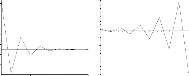
According to the convergence criterion given above, the Laurent expansion

should converge for z = Z = 3 and diverge for z =7. Entering P(3) yields

the plot on the left of Figure 5.6, while P(7) generates the plot on the right.

P(3); P(7);

0.36

0.38

0.4

0.42

810

–2

246810

Figure 5.6: Left plot: Convergence for z =Z = 3; Right: Divergence for z =7.

The Laurent expansion clearly converges to the exact f value for z = 3 and

diverges for z =7.”

5.5 Conformal Mapping

The relation ω = f(z) describes a mapping of points in the complex z-plane

into corresponding points in the ω-plane. If f(z) is a single-valued function of

z = x + iy, each point in the z-plane maps into a single point in the ω-plane.

If f(z) is a multi-valued function with n branches, each point in the z-plane

maps into n points in the ω-plane. For example, ω =z

1/2

has two branches with

each point in the z-plane producing two points in the ω-plane. The mapping

from the z-plane can be made one to one by introducing a branch cut in the

z-plane and restricting our attention to a single branch of the function, usually

referred to as the principal branch.Forω = f(z)=z

1/2

, the principal branch

is traditionally obtained by introducing a branch cut along the negative x-axis

and restricting the polar angle θ to the range −π<θ<π. The principal branch

of z

1/2

maps only into the u>0halfoftheω-plane, i.e., the polar angle in this

plane is restricted to the range −π/2 <θ<π/2.

If f(z) is analytic (and df/dz =0)atapointz

in the z-plane, the angle be-

tween two curves intersecting at z

is not changed on transforming to the corre-

sponding point ω

in the ω-plane, even though the shapes of the two curves will

generally change. Transformations which have this angle-preserving property

are called conformal transformations or conformal mapping. The orthogonality

of the equipotential and ﬁeld lines in potential problems is preserved under a

5.5. CONFORMAL MAPPING 209

conformal mapping. It is not surprising therefore that a solution of Laplace’s

equation in one plane remains a solution in the other.

Conformal mapping may be used for solving 2-dimensional potential prob-

lems. Suppose that we are given a potential problem with a somewhat compli-

cated boundary condition. We then try to transform the problem to a new plane

where the boundary conﬁguration is simpler. On solving this simpler situation,

we can transform the results back to the original plane, thus determining the

ﬁeld and potential conﬁguration for the original problem.

Many important conformal mappings, such as in the following recipe, can

be discovered by experimenting with diﬀerent mathematical forms.

5.5.1 Field Around a Semi-inﬁnite Plate

If all the ways I have been along were marked on a map and joined

up with a line, it might represent a minotaur.

Pablo Picasso, Spanish artist, (1881–1973)

In this recipe, I will use the mapping ω =

√

z to determine the equipoten-

tials and electric ﬁeld (represented by ﬁeld lines and by vectors) in the vicinity

of a thin semi-inﬁnite grounded (held at zero potential) conducting plate. The

problem can be treated as 2-dimensional with the cross-section of the plate as

schematically shown in Figure 5.7.

semi-infinite plate

infinity -->

<-- -infinity

Figure 5.7: Cross-section of the thin semi-inﬁnite plate.

The VectorCalculus package is loaded, because the Gradient command will

be used to calculate the electric ﬁeld vector



E = −∇u,withu the potential.

restart: with(plots): with(VectorCalculus):

The given mapping function is entered.

w:=sqrt(z);

w :=

√

Before solving the problem, it is instructive to see the eﬀect of the trans-

formation w = u + iv=

√

z =

√

x + iy on the grid lines x = c

, y = c

,where

and c

are real constants. Forming the inverse transformation z = w

and

separating into real and imaginary parts, we have x = u

−v

and y =2uv.A

grid line x = c

is mapped into that portion of the hyperbola u

− v

= c

for

which u>0, while y =c

is mapped into a branch of the rectangular hyperbola

2 uv=c

, the branch depending on whether c

is positive or negative.

210 CHAPTER 5. COMPLEX VARIABLES

A graphical conﬁrmation of the transformation of grid lines from the z-

plane to the ω-plane can be generated by applying the following conformal

command to the grid lines in a particular region of the z-plane , e.g., the region

−2 ≤ x ≤ 2, −2 ≤ y ≤ 2.

conformal(w,z=-2-2*I..2+2*I,grid=[14,14],numxy=[100,100],

color=[red,blue],scaling=constrained,labels=["u","v"]);

The grid option is used to specify the number of grid lines in both the x

and y directions, the default being 11 × 11. The option numxy=[m,n],with

m = 100 and n = 100 here, is employed to specify the number of points to be

plotted in each grid line, with m points in the x direction and n points in the

y direction. The default is 15 points in each direction. The transformed curves

corresponding to constant x will be colored red, while those corresponding to

constant y are colored blue. The scaling is constrained and labels u, v, added.

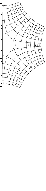
The rectangular region −2 ≤ x ≤ 2, −2 ≤ y ≤ 2inthez-plane maps into

thecurvedgridregionintheω-plane shown in Figure 5.8.

–1.5

1.5

Figure 5.8: Rectangular grid in z-plane maps into curved grid in ω-plane.

As expected, the curves y = c

for c

> 0 map into the rectangular hyperboli

in the ﬁrst quadrant (u>0, v>0) of the w-plane, while those for c

< 0

map into rectangular hyperboli in the fourth quadrant (u>0, v<0). The

x = c

lines map into the hyperbolic curves in the ﬁgure which intersect the

rectangular hyperboli. The 90

◦

angle between grid lines is preserved by the

conformal transformation.

Now, let’s tackle the problem of the semi-inﬁnite grounded conducting plate.

Setting z =x + iy, ω takes the following form,

z:=x+I*y: w:=w;

w :=

√

x + yI

which can be split into real and imaginary parts by applying the complex eval-

uation (evalc) command.

5.5. CONFORMAL MAPPING 211

w2a:=evalc(w) assuming y>0; w2b:=evalc(w) assuming y<0;

w2a :=





+ y

+2x





+ y

− 2 x

w2b :=





+ y

+2x

−





+ y

− 2 x

w2a shows the form of ω for y>0, while w2b applies when y<0. The potential

u relevant to our problem is obtained by removing the imaginary part from w2a.

u:=remove(has,w2a,I);

u :=





+ y

+2x

The electric ﬁeld lines for y>0andy<0 are obtained in v2a and v2b by

selecting the imaginary parts of w2a and w2b, respectively, and dividing by i.

v2a:=select(has,w2a,I)/I: v2b:=select(has,w2b,I)/I:

The electric ﬁeld vector



E = −∇u is calculated in Cartesian coordinates.

E:=-Gradient(u,’cartesian’[x,y]);

E := −

2 x



+ y





+ y

+2x

−





+ y

+2x



+ y

Now, let’s plot the results. A thick blue line is plotted between (−2, 0) and

(0, 0) to represent a portion of the semi-inﬁnite plate.

gr1:=plot([[-2,0],[0,0]],style=line,color=blue,thickness=4):

The fieldplot command is used to plot the electric ﬁeld vector



E, the vectors

being represented by thick red arrows.

gr2:=fieldplot([E[1],E[2]],x=-2..2,y=-2..2,arrows=THICK,

grid=[10,10],color=red):

A functional operator G is formed to produce a contour plot of any input function

V ,thecolorC of the curves to be speciﬁed. The range is taken to be x = −2

to2andy = −2 to 2. The contours are chosen to be V =0, 0.2, 0.4, ..., 2.

G:=(V,C)->contourplot(V,x=-2..2,y=-2..2,contours=

[seq(0.2*n,n=0..10)],grid=[60,60],color=C):

Using G, the equipotentials (u =const.) and electric ﬁeld lines are plotted

together, along with the plate, using the display command.

display({gr1,G(u,green),G(v2a,red),G(v2b,red)});

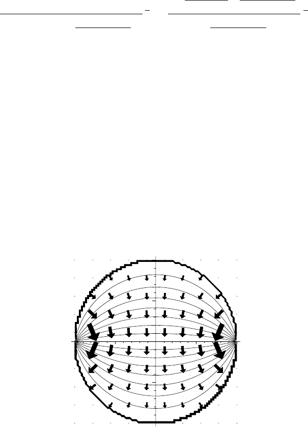
On the computer screen, the equipotentials are colored green and the electric

ﬁeld lines red. The corresponding black and white version is shown on the left

of Figure 5.9.

The semi-inﬁnite plate is represented by the thick horizontal line between

x=−2 and 0. The equipotentials are the family of parabolas opening to the left,

the closest one to the plate being for φ =0.2, the next furthest one for φ =0.4,

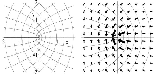
212 CHAPTER 5. COMPLEX VARIABLES

and so on. The electric ﬁeld lines are the family of parabolas opening to the

right. Naturally, they intersect the equipotential at right angles. This includes

the plate which is the zero equipotential. The electric ﬁeld lines terminate on

the surface charge on the plate.

Figure 5.9: Equipotentials and (a) ﬁeld lines (left plot), (b) ﬁeld vectors (right).

The ﬁeld lines convey the sense of the electric ﬁeld but do not indicate how the

ﬁeld strength varies with distance from the plate. To this end, the following

display command is used to superimpose the equipotentials and the electric

ﬁeld (



E) vectors.

display({gr1,gr2,G(u,green)});

It can be seen from the resulting picture shown on the right of Figure 5.9 that

the electric ﬁeld is strongest near the edge of the plate, i.e., near the tip of the

thick line in the ﬁgure.

5.5.2 A Clever Transformation

We are obliged to regard many of our original minds as crazy at least

until we have become as clever as they are.

G. C. Lichtenberg, German physicist, philosopher, (1742–99)

An inﬁnitely long conducting cylinder of unit radius, with its axis horizon-

tal, has its upper-half held at the potential Φ = +V and its lower-half held

at Φ = −V , the two halves being separated by an inﬁnitesimally thin layer of

insulation. What are the equipotentials and electric ﬁeld inside the cylinder?

The fact that this problem is 2-dimensional in nature, and has a certain

symmetry to it, allows us to solve it rather easily by using a conformal trans-

formation approach. Loading some needed library packages,

restart: with(plots): with(VectorCalculus):

5.5. CONFORMAL MAPPING 213

the complex variable z = x + iy is entered. As will be seen, the mapping

w = ln((1 + z)/(1 − z)), which is inputted, will transform the original circular

boundary value problem into a planar boundary value problem which can be

solved by inspection.

z:=x+I*y: w:=ln((1+z)/(1-z));

w := ln(

x + yI+1

−x − yI+1

)

The complex function w = u + iv is split into real and imaginary parts with

the complex evaluation command, and u and v separately extracted with the

remove and select commands, respectively.

w:=simplify(evalc(w));

w :=

ln(

+2x+1+y

−2 x+1+y

)+arctan(

2 y

−2 x+1+y

, −

−1+y

−2 x+1+y

) I

u:=remove(has,w,I); v:=select(has,w,I)/I;

u :=

ln(

+2x +1+y

− 2 x +1+y

)

v := arctan(

2 y

− 2 x +1+y

, −

− 1+y

− 2 x +1+y

)

Recognizing that the ﬁrst argument of the arctangent in v is the numerator

and the second argument the denominator, v is expressed in a more familiar

mathematical form by using the operand (op) command.

v:=arctan(op(1,v)/op(2,v));

v := −arctan(

2 y

− 1+y

)

Since v satisﬁes Laplace’s equation, it can be taken as the potential. To see

how the potential on the circular boundary transforms under the action of w,

let’s make the algebraic substitution y

=1− x

in w.

w2:=algsubs(yˆ2=1-xˆ2,w);

w2 :=

ln(

2 x +2

−2 x +2

) + arctan(

2 y

−2 x +2

, 0) I

The result w2 is simpliﬁed in w3a, assuming that y>0andx<1, and in w3b,

assuming that y<0andx<1.

w3a:=simplify(w2) assuming y>0,x<1;

w3a := −

ln(−x +1)+

ln(x +1)+

Iπ

w3b:=simplify(w2) assuming y<0,x<1;

w3b := −

ln(−x +1)+

ln(x +1)−

Iπ

The select command is used to extract the imaginary parts of w3a and w3b

which are then divided by i in v2a and v2b, respectively.

v2a:=select(has,w3a,I)/I; v2b:=select(has,w3b,I)/I;

214 CHAPTER 5. COMPLEX VARIABLES

v2a :=

v2b := −

The upper (lower) surface of the split cylinder, which is at the potential +V

(−V ), maps into the inﬁnite plane v2a =+π/2(v2b = −π/2). The region

inside the split cylinder maps into the region between these inﬁnite planes.

The potential problem in the w plane is easily solved. By inspection, the

equipotentials must be parallel planes lying between v =+π/2and−π/2, v =0

(the u-axis) corresponding to the zero potential. Analytically, the potential

must be given by Φ = (2 v/π)V ,sincev = π/2 generates the equipotential

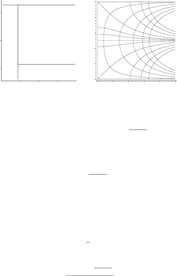
Φ=V , and so on. A picture of the equipotentials in the w plane are generated

for V =1 with the contourplot command.

contourplot(2*Y/Pi,X=-2..2,Y=v2b..v2a);

–1

–2 2

Figure 5.10: Planar equipotentials in the w-plane.

Entering Φ = 2 Vv/π generates the potential in terms of x and y, i.e., in the

z-plane. It can be converted to polar form if so desired, as in Φ2.

Phi:=2*V*v/Pi;

Φ:=−

2 V arctan(

2 y

− 1+y

)

Phi2:=simplify(subs({x=r*cos(theta),y=r*sin(theta)},Phi));

Φ2 := −

2 V arctan(

2 r sin(θ)

−1+r

)

The electric ﬁeld expression follows on calculating



E = −∇Φ.

E:=-Gradient(Phi,’cartesian’[x,y]);

5.5. CONFORMAL MAPPING 215

E := −

8Vyx

−1+y

)

(1+

4 y

−1+y

)

)π

2V(

−1+y

−

4 y

−1+y

)

(1+

4 y

−1+y

)

)π

A normalized piecewise potential function is formed, made up of Φ/V inside

the unit circle and zero outside.

pot:=piecewise(xˆ2+yˆ2<1,Phi/V,xˆ2+yˆ2>1,0);

The x and y components of the normalized electric ﬁeld are also put into a

similar piecewise form in E1 and E2 .

E1:=piecewise(xˆ2+yˆ2<1,E[1]/V,xˆ2+yˆ2>1,0):

E2:=piecewise(xˆ2+yˆ2<1,E[2]/V,xˆ2+yˆ2>1,0):

The normalized equipotentials are plotted with the contourplot command.

cp:=contourplot(pot,x=-1..1,y=-1..1,grid=[80,80],

contours=15):

The normalized electric ﬁeld vectors are plotted using the fieldplot command.

fp:=fieldplot([E1,E2],x=-1..1,y=-1..1,grid=[10,10],

arrows=THICK,color=red):

The two graphs, cp and fp, are superimposed to produce Figure 5.11.

display({cp,fp},scaling=constrained);

–1

–1 1

Figure 5.11: Equipotentials and electric ﬁeld vectors for the split cylinder.

Although this split cylinder problem was easily solved using a conformal trans-

formation, it should be noted that this approach is limited in its usefulness,

being applicable to two-dimensional potential problems of relatively simple ge-

ometry or symmetry.

216 CHAPTER 5. COMPLEX VARIABLES

5.5.3 Schwarz–Christoﬀel Transformation

Physical concepts are free creations of the human mind, and are not,

however it may seem, uniquely determined by the external world.

Albert Einstein, German-American physicist, Evolution of Physics, 1938

To this point, the conformal transformations have been drawn out of “thin air”.

A systematic approach for obtaining many speciﬁc transformations is to apply

the general Schwarz–Christoﬀel transformation which can be used to transform

the inside

of a closed polygon in the z = x + iy plane into the upper half of

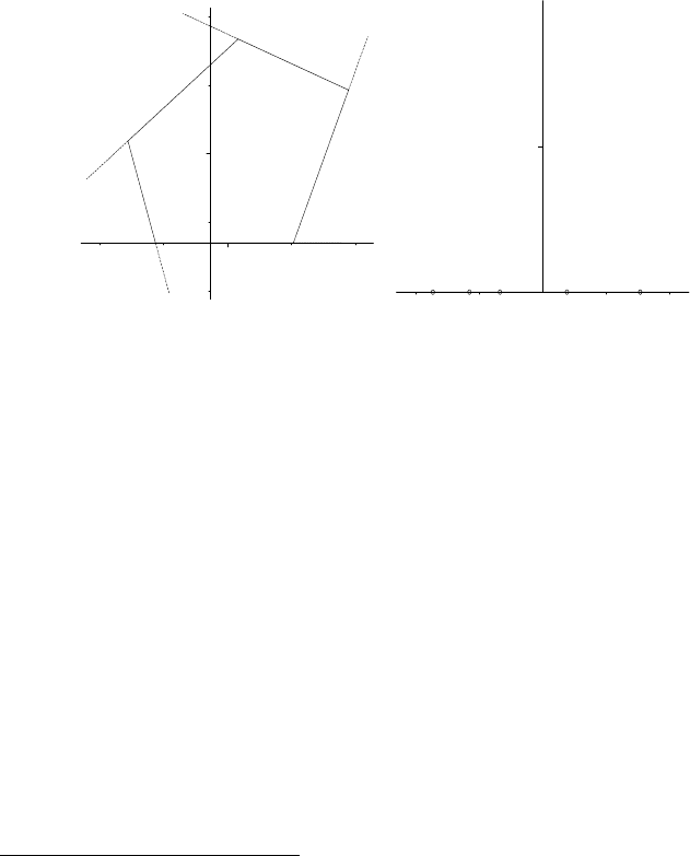
the w =u + iv plane. Referring to Figure 5.12, the vertices of the polygon are

z Plane

Inside

α0

α4

α3

α2

α1

w Plane

InsideInside

b4b3b2b1b0

Figure 5.12: Schwarz–Christoﬀel transformation.

labeled a0, a1,..., the corresponding exterior angles α0, α1,..., and the trans-

forms of the vertices to the w plane b0, b1,.... Traversing the exterior of the

polygon in a counterclockwise sense, so that the interior of the polygon is to the

left, angles which correspond to turning further to the left are taken as positive,

while turns to the right are regarded as negative.

The Schwarz–Christoﬀel (S-C) transformation which maps the interior of

the polygon in the z plane onto the upper-half of the w plane and the boundary

of the polygon onto the real (u) axis is given by

z = A



(w − b0)

−α0/π

(w − b1)

−α1/π

···(w − bn)

−αn/π

dw + B, (5.10)

where A and B are arbitrary complex constants. Note the following facts:

• Any three of the points b0, b1,...,bn may be chosen at will. We can place

b0 at inﬁnity which removes the ﬁrst factor in (5.10).

• A and B are adjusted to ﬁx the polygon size, orientation, and position.

• Inﬁnite open polygons are regarded as limiting cases of closed polygons.

The method can be extended to map the outside of the polygon, see, e.g., [MF53].

5.5. CONFORMAL MAPPING 217

As a simple example, let’s determine the S-C transformation which maps

the interior of the semi-inﬁnite rectangular strip shown on the left of Figure 5.13

into the upper-half of the w plane. Then, this transformation will be used to

plot the equipotentials and lines of force inside a straight slit, with the same

geometry, cut in an inﬁnite conducting sheet.

a0 ---> infinityStrip

a2 = 0

a1 = ih

α2 = π/2

α1 = π/2

Figure 5.13: Geometry (left) and equipotentials and ﬁeld lines (right) for strip.

The inﬁnite strip can be regarded as the limit of a triangle with vertices a0 →∞,

a1 = ih, and a2 = 0. The exterior angles then are α0=π, α1=π/2, and

α2=π/2. Choosing b0 = ∞,b1=−1, and b2 = 1, the S-C transformation is

given by z =A



(w +1)

−1/2

(w − 1)

−1/2

dw + B =



(1/

√

− 1) dw + B.

After loading the plots package, needed for the contour plot,

restart: with(plots):

the integral in the S-C transformation is explicitly carried out.

Z:=A*int(1/sqrt(wˆ2-1ˆ2),w)+B;

Z := A ln(w +

√

− 1) + B

Now, when z = a2 = 0, then w = b2 = 1. Similarly, when z =a1=ih,then

w =b1=−1. These two boundary conditions are entered,

bc1:=eval(Z,w=1)=0; bc2:=eval(Z,w=-1)=I*h;

bc1 := B =0 bc2 := AπI + B = hI

and solved for the constants A and B.

sol:=solve({bc1,bc2},{A,B});

sol := {A =

,B=0}

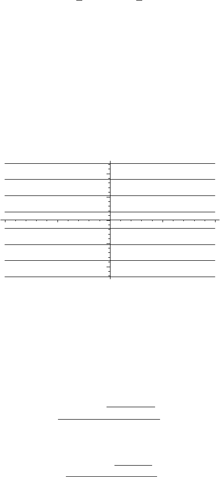
On assigning the solution, the S-C transformation is given by Z.

assign(sol): Z:=Z;

Z :=

h ln(w +

√

− 1)