Enns R.H. Computer Algebra Recipes for Mathematical Physics

Подождите немного. Документ загружается.

198 CHAPTER 5. COMPLEX VARIABLES

The value of the integral follows on multiplying r by 2 πi and applying the

complex evaluation command to simplify the answer to a real number.

V:=evalc(2*Pi*I*r);

V :=

√

As a check, we can directly evaluate the integral using Maple’s int command.

This is done in the next two command lines, the resulting number being the

same as that obtained above using contour integration.

I1:=Int(integrand,z=-infinity..infinity);

I1 :=



∞

−∞

1+z

check:=value(I1);

check :=

√

If the semi-circular contour had been chosen to be in the lower-half z-plane,

exactly the same answer would be generated using the poles below the real

axis, provided that the result is multiplied by −1 to take into account that the

contour then is taken in a clockwise sense, rather than counterclockwise.

5.3.2 Poles on the Contour

There are many paths to the top of the mountain,

but the view is always the same.

Chinese Proverb

In the previous example, the poles of the integrand were either deﬁnitely inside

or outside the path chosen for the contour integration. Suppose that we want

to evaluate the integral I =



∞

−∞

cos(x) dx/(a

− x

)witha real. The inﬁnite

limits suggest a semi-circular contour C in the complex z-plane with the ﬂat

portiononthereal(x) axis. But the integrand has two simple poles lying right

on C at x = ±a. To apply Cauchy’s residue theorem, the poles must be def-

initely inside or outside the chosen contour. So what do we do? A standard

approach is to “indent” the contour in the vicinity of each pole, taking a small

semi-circular “detour” around the pole which either puts the pole inside or out-

side the contour. Then one performs the contour integration using the residue

theorem, and afterwards lets the radii of the small semi-circles go to zero. As

an illustration of this method, let’s evaluate the above integral I.

The plottools library package is again loaded so the various semi-circles can

be drawn for the indented contour.

restart: with(plots): with(plottools):

Instead of tackling I directly, let’s consider the integral



dz/(a

−z

), with

z the complex variable. At the end of the calculation the real integral I can be

5.3. DEFINITE INTEGRALS 199

obtained by taking the real and imaginary parts. The integrand of the complex

closed contour integral is now entered.

integrand:=exp(I*z)/(aˆ2-zˆ2);

integrand :=

(zI)

− z

The integrand’s poles can be extracted by applying the discontinuity command.

pole:=discont(integrand,z);

pole := {a, −a}

To draw the indented semi-circular contour, let’s take the poles to be at ±1by

setting a = 1. The small semi-circle around each pole is given a radius r =0.2,

and the larger semi-circle which completes the path is given a radius R =2.

R:=2: r:=0.2: a:=1:

An operator A is formed to draw a thick red semi-circle of arbitrary radius r

around a speciﬁed point (x, 0) on the real axis.

A:=(x,r)->arc([x,0],r,0..Pi,color=red,thickness=2):

Using A, a large semi-circle of radius R centered on the origin is produced in

A1, and a small semi-circle of radius r around each pole in A2 and A3.

A1:=A(0,R): A2:=A(pole[1],r): A3:=A(pole[2],r):

In B, a thick red line is drawn along the real axis between, x= −R and −a −r,

between −a + r and a −r, and between a + r and R.

B:=plot([[[-R,0],[-a-r,0]],[[-a+r,0],[a-r,0]],

[[a+r,0],[R,0]]],style=line,color=red,thickness=2):

In C, the two poles are plotted as size 16 blue circles.

C:=pointplot([[pole[1],0],[pole[2],0]],symbol=circle,

symbolsize=16,color=blue):

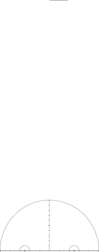
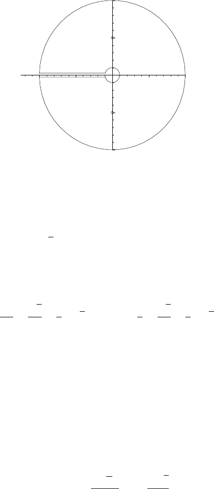
The graphs are superimposed, generating the full contour shown in Figure 5.4.

display({A1,A2,A3,B,C},scaling=constrained,

view=[-R..R,0..R],tickmarks=[2,2],labels=["x","y"]);

–2 2

Figure 5.4: Semi-circular contour indented around the two poles on the x-axis.

200 CHAPTER 5. COMPLEX VARIABLES

Note that I have chosen to indent the small semi-circles around each pole in

such a way that both poles lie outside the contour C. So the line integral around

C will yield zero, since no poles lie inside C. I could just as well have chosen

to indent the small semi-circles in such a way that both poles were inside the

contour, or even so that one pole was inside and the other outside. As you may

verify, the ﬁnal answer is the same, irrespective of the choice of indentation.

The quantities a and r are now unassigned. On each small semi-circle, the

complex variable will be written as Z =re

iθ

a:=’a’: r:=’r’: Z:=r*exp(I*theta):

For our choice of C, starting at the point (−R, 0) the complete counterclockwise

contour integral will be as follows:

− z

)

=0 =



−a−r

−R

− x

)



i(−a+Z)

iZ dθ

− (−a + Z)

)



a−r

−a+r

− x

)



i(a+Z)

iZ dθ

− (a + Z)

)



a+r

− x

)



iRe

iθ

iRe

iθ

dθ

− (Re

iθ

)

In the limit that R →∞and r → 0, the sum of the ﬁrst, third, and ﬁfth

integrals on the right-hand side of 0 will yield



∞

−∞

dx/(a

− x

). Taking

the real part will produce the original integral



∞

−∞

cos(x) dx/(a

− x

), whose

value we are trying to determine.

Let’s look at the last integral on the right-hand side, which is written as



iR cos θ−R sin θ

iRe

iθ

dθ

− R

2iθ

)

Since the large semi-circle is in the upper-half z-plane, sin θ>0. Therefore,

as R →∞, the integrand → 0 and the integral contribution is zero. Finally,

we have to evaluate the second and fourth integrals on the right-hand side. A

function F is formed for substituting z = ±a + Z into the integrand.

F:=n->subs(z=pole[n]+Z,integrand):

Theﬁrstpoleextractedwas+a (the ordering varies from one run to the next),

so F(1) is used to form the fourth integral and simplify it.

I1:=simplify(Int(F(1)*I*Z,theta=Pi..0));

I1 := −I



((a+re

(θI)

) I)

2 a + re

(θI)

dθ

Taking the limit of I1 at r =0 completes the evaluation of the integral in I1b.

I1b:=limit(I1,r=0);

I1b :=

(aI)

Using F(2), the second integral is similarly formed in I2 and evaluated in I2b.

5.3. DEFINITE INTEGRALS 201

I2:=simplify(Int(F(2)*I*Z,theta=Pi..0));

I2 := −I



((−a+re

(θI)

) I)

−2 a + re

(θI)

dθ

I2b:=limit(I2,r=0);

I2b :=

−1

(−Ia)

The two integral terms are added and simpliﬁed assuming that a is real.

terms:=simplify(I1b+I2b) assuming a::real;

terms := −

π sin(a)

The answer to the original real integral is just minus the above output.

answer:=Int(cos(x)/(aˆ2-xˆ2),x=-infinity..infinity)=-terms;

answer :=



∞

−∞

cos(x)

− x

dx =

π sin(a)

5.3.3 An Angular Integral

Science is an integral part of culture. ... It’s one of the glories of

the human intellectual tradition.

Stephen Jay Gould, American scientist, (b. 1941)

Integrals whose integrands are rational functions of cos θ and sin θ in the range

of integration can be evaluated by making the transformation z =e

iθ

.Ifθ varies

from0to2π, the integration in the complex z-plane will be counter-clockwise

around a circle of unit radius. As an example, consider

J =



2π

sin

θdθ

(5 + 4 cos θ)

For variety, let’s load the Student[Calculus1] package, which contains two useful

commands, Integrand and Roots, which haven’t been used yet.

restart: with(Student[Calculus1]):

The integral J is now entered and, as a check on the contour integration, eval-

uated directly with the value command.

J:=Int(sin(theta)ˆ2/(5+4*cos(theta)),theta=0..2*Pi);

J :=



2 π

sin(θ)

5 + 4 cos(θ)

dθ

check:=value(J);

check :=

A contour integration should yield the value π/4forJ. To carry out this

integration, note that sin θ =(e

iθ

− e

−iθ

)/(2i)=(z − 1/z)/(2i)andcosθ =

iθ

+ e

−iθ

)/2=(z +1/z)/2. These two transformations are entered.

202 CHAPTER 5. COMPLEX VARIABLES

sin(theta):=(z-1/z)/(2*I); cos(theta):=(z+1/z)/2;

sin(θ):=

−1

I (z −

) cos(θ):=

2 z

Using the Integrand command to extract the integrand of J and using the fact

that dθ = dz/(iz), the integrand of the contour integral is as follows.

integrand:=simplify(Integrand(J)/(I*z));

integrand :=

I (z

− 1)

(5 z +2z

+2)

The Roots command is used to determine the zeros of the reciprocal of the

integrand, and thus the poles of the integrand.

R:=Roots(1/integrand);

R := [−2,

−1

, 0]

There are three poles, viz., two simple poles at z = −2andz = −1/2anda

second order pole at z =0. Since the contour C is a unit circle in the z-plane,

the pole at z = −2 will not contribute to the answer since it’s outside C.The

residue of the integrand at the two poles inside C is calculated in r1 and r2 .

r1:=residue(integrand,z=R[2]); r2:=residue(integrand,z=R[3]);

r1 :=

I r2 :=

−5

By Cauchy’s residue theorem, the value of the integral J is just 2 πi times the

sum of the two residues. The answer is π/4 as expected.

answer:=2*Pi*I*(r1+r2);

answer :=

5.3.4 A Branch Cut

Trust everybody, but cut the cards.

Finley Peter Dunne, American journalist, (1867–1936)

Cauchy’s residue theorem is built on the assumption that the integrand f(z)

in the contour integral



f(z) dz is a single-valued function. What if f(z)is

multi-valued with more than one mathematical branch? The answer is to choose

a contour which keeps f(z) on a single branch. Typically, a line is drawn in

the complex z-plane, called a branch cut, which the contour is not permitted to

cross in order to keep f(z) single-valued. Section 5.5 will elaborate on this.

To see how the procedure is implemented for a speciﬁc integral, consider

J =



∞

√

xdx

1+x

. The corresponding complex integral is



(

√

z/(1 + z

)) dz,

which has a double-valued integrand because of the

√

z factor. The branch cut

will be taken from z = 0 (the branch point) to −∞ along the negative x-axis.

(The branch cut could be taken in any direction from z =0 to ∞.) The contour

5.3. DEFINITE INTEGRALS 203

C is chosen to consist of an inner circle of radius  and an outer circle of radius

R (both centered on the origin) joined by horizontal lines a distance η above

and below the branch cut. Ultimately, we let both  and η → 0andR →∞.

In order to draw the circular arcs in C, the plottools library package is ﬁrst

loaded. The complex integrand is then entered.

restart: with(plots): with(plottools):

integrand:=sqrt(z)/(1+zˆ2);

integrand :=

√

1+z

Before drawing C, let’s use the singular command to extract the singularities

of the integrand, needed for the application of Cauchy’s residue theorem.

pole:=singular(integrand);

pole := {z = I}, {z = −I}

There are two singular points at z = i and z =−i, corresponding to the locations

of two simple poles. The operand command, op, is now used to separately obtain

the locations, z1 and z2 , of the two poles.

z1:=op([1,2],pole[1]); z2:=op([1,2],pole[2]);

z1 := I z2 := −I

The pole locations may be converted into polar form.

z1_polar:=convert(z1,polar); z2_polar:=convert(z2,polar);

polar := polar(1,

) z2

polar := polar(1, −

)

The poles lie on a circle of radius 1 at the polar angles θ=+π/2and−π/2. To

schematically draw the contour, let’s set R =2,  =0.2, and η =0.05.

R:=2: epsilon:=0.2: eta:=0.05:

Thick red circular arcs of radius  and R, respectively, are drawn in A1 and A2.

A1:=arc([0,0],epsilon,Pi-0.2..-Pi+0.2,color=red,thickness=2):

A2:=arc([0,0],R,Pi-0.02..-Pi+0.02,color=red,thickness=2):

A thick blue line is drawn along the real axis between x = −R − 0.5 and the

origin to represent the branch cut.

B:=plot([[-R-0.5,0],[0,0]],style=line,color=blue,thickness=3):

Red lines are drawn between (−R,η), (−,η) and between (−R,−η), (−,−η).

B2:=plot([[[-R,eta],[-epsilon,eta]],[[-R,-eta],

[-epsilon,-eta]]],style=line,color=red,thickness=2):

The two poles are represented by size 16 blue circles,

C:=plot({[0,z1/I],[0,z2/I]},style=point,symbol=circle,

symbolsize=16,color=blue):

and the textplot command is used to add labels to the ﬁgure.

tp:=textplot([[-1.9,-.15,"a"],[-1.9,.15,"b"],[-.25,.15,"c"],

[-.25,-.15,"d"],[-2.3,.1,"cut"]]):

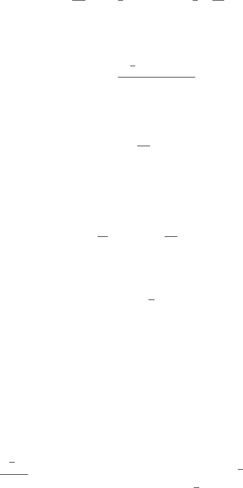
The six plots are superimposed, the resulting picture being shown in Figure 5.5.

204 CHAPTER 5. COMPLEX VARIABLES

display({A1,A2,B,B2,C,tp},scaling=constrained,

view=[-R-0.5..R,-R..R],labels=["x","y"]);

cut

–1

–1 1

Figure 5.5: Closed contour around branch cut (stretching from z =0 to −∞).

The complete contour C consists of four legs, viz., a → b, b → c, c → d,and

d → a. Traversing C counter-clockwise, in the limit that η → 0, the increase of

2 π in θ in going from a to b is canceled out by the −2 π contribution in going

from c to d. Since the net angular change is zero, f (z) remains single-valued.

Multi-valuedness of f(z)=

√

z/(1+z

) only occurs if the net change in θ exceeds

2 π.Sincef(z) is single-valued, Cauchy’s residue theorem can be applied. The

poles lie inside C, so the line integral around C will yield a non-zero result.

Let’s calculate the residues of the integrand at the two poles.

r1:=residue(integrand,z=z1); r2:=residue(integrand,z=z2);

r1 :=

−1

I (

√

2) r2 :=

I (

√

−

√

Now let’s look at each contribution to the line integral in the limit that η → 0.

(a) The integral I

a→b



−π

(iR

3/2

3iθ/2

/(1 + R

2iθ

)) dθ → 0asR →∞.

(b) I

b→c





1/2

3πi/2

/(1 + r

2πi

)) dr → iJ as  → 0andR →∞.

c→d



−π

(i

3/2

3iθ/2

/(1 + 

2iθ

)) dθ → 0as → 0.

(d) I

d→a





1/2

−3πi/2

/(1 + r

−2πi

)) dr → iJ as  → 0andR →∞.

Since these four contributions add up to 2 iJ, the original integral must equal

2 πi times the sum of the two residues divided by 2 i.

answer:=Int(sqrt(x)/(1+xˆ2),x=0..infinity)

=evalc(2*Pi*I*(r1+r2)/(2*I));

answer :=



∞

√

1+x

dx =

√

As a check, we apply the value command to the left-hand side of answer,

5.4. LAURENT EXPANSION 205

check:=value(lhs(answer));

check :=

√

obtaining exactly the same result as in the contour integration.

5.4 Laurent Expansion

Using Cauchy’s integral formula, one can prove Laurent’s theorem:Ifg(z)is

regular in an annular region R between two concentric circles with center z

then g(z) may be represented in R by a Laurent expansion

g(z)=

∞



n=−∞

(z − z

)

, with a

2 πi

g(z) dz

(z − z

)

n+1

, (5.7)

C being any simple closed path encircling z

counter-clockwise within R.

If g(z) has a ﬁnite number of terms with negative exponents, it’s behavior is

dominated as z approaches z

by the term with the largest negative exponent.

If, e.g., it has the form

g(z)=

−n

(z − z

)

−(n−1)

(z − z

)

n−1

+ ···+

−1

(z − z

)

+ a

(z −z

)+···, (5.8)

then it has a pole of order n at z = z

. Note that if g(z) in (5.8) is multiplied

by (z − z

)

, the result then diﬀerentiated n − 1 times and z set equal to z

then the coeﬃcient a

−1

is just the residue of the nth order pole, i.e.,

−1

(n − 1)!



n−1

[(z − z

)

g(z)]

n−1



z = z

. (5.9)

If g(z) has an inﬁnite number of terms with negative exponents, it is said to

have an essential singularity at z =z

. For example, g(z)=e

=1+

+ ···

has an essential singularity at z =0.

Instead of doing the contour integrations in (5.7), the coeﬃcients a

can

often be more easily obtained by considering the Taylor series of (z −z

)

g(z).

5.4.1 Ms. Curious Meets Mr. Laurent

Isn’t life a series of images that change as they repeat themselves?

Andy Warhol, American pop artist, (1928–87)

Jennifer has posed the following question for her complex variables class:

Keeping 10 terms, determine the Laurent expansion of f =cos(z) e

z−2z

about z = 0. Identify the singularity and give the region of convergence of the

series. Determine the residue of f at the singularity from the series. Conﬁrm

the value of the residue by alternate means.

Here is the solution presented by Ms. Curious, expressed in her own words.

206 CHAPTER 5. COMPLEX VARIABLES

“The number N of terms to be retained in the series is set equal to 10.

restart: N:=10:

Since the numerator remains ﬁnite there, clearly f has a second-order pole at

z = 0. To obtain the Laurent series about this singularity, I will enter the

coeﬃcient of 1/z

in G.

G:=cos(z)*exp(z-2*zˆ2);

G := cos(z) e

(z−2 z

)

Then G is Taylor expanded in powers of z to order N , and the order of term

removedwiththeconvert(g,polynom) command.

g:=taylor(G,z,N);

g:=convert(g,polynom);

g := 1+z − 2 z

−

− z

−

1217

630

841

2520

23617

22680

The Laurent expansion follows on dividing g by z

and expanding the result.

LS:=expand(g/zˆ2);

LS :=

− 2 −

7 z

11 z

79 z

− z

−

1217 z

630

841 z

2520

23617 z

22680

The Laurent expansion LS converges for all values of z = 0. By inspecting

the series and recalling that the residue is the coeﬃcient of the 1/z term, the

residue of f at z = 0 is 1. It should be noted that the Laurent series can also

be obtained by loading the numapprox library package, applying the laurent

command to G/z

as in check1 , and removing the order of term as in LSb.

with(numapprox):

check1:=laurent(G/zˆ2,z=0,N);

LSb:=convert(check1,polynom);

LSb :=

− 2 −

7 z

11 z

79 z

− z

−

1217 z

630

841 z

2520

23617 z

22680

The residue of f(z)atz = 0 can also be obtained by diﬀerentiating z

f or G

once (since the singularity is a pole of order 2) with respect to z, evaluating the

result at z =0, and dividing by 1!

r1:=eval(diff(G,z),z=0)/1!;

r1 := 1

An even simpler method of determining the residue of f = G/z

at z =0 is to

use the residue command.”

r1b:=residue(G/zˆ2,z=0);

r1b := 1

5.4. LAURENT EXPANSION 207

5.4.2 Converge or Diverge?

I shall be telling this with a sigh, Somewhere ages and ages hence:

Two roads diverged in a wood, and I –

I took the one less traveled by, And that has made all the diﬀerence.

Robert Frost, American poet, The Road Not Taken (1874-1963)

Jennifer has given a second quiz question on the Laurent expansion.

Find the Laurent series for f = z

/((z − 1)

(z +3) aboutz =1. Determine

the residue and the region of convergence. Conﬁrm the latter by creating plots

for diﬀerent z values which show convergence and divergence.

Again, Ms. Curious will present her recipe for solving this problem.

“The numapprox package is loaded so that the laurent command can be

used. The given function f is then entered. It has a second order pole at z =1

and a ﬁrst order pole at z =−3.

restart: with(plots): with(numapprox):

f:=zˆ2/((z-1)ˆ2*(z+3));

f :=

(z − 1)

(z +3)

An arrow operator L is formed for calculating the Laurent expansion of f

about z =1 to terms of order (z −1)

. For example, for N =5, the Laurent

series has the explicit form given in LS.

L:=N->laurent(f,z=1,N): LS:=L(5);

LS :=

(z − 1)

−2

(z − 1)

−1

−

256

(z − 1) +

1024

(z − 1)

−

4096

(z − 1)

16384

(z − 1)

+O((z −1)

)

By examining the (z −1)

−1

term, I can see that the residue is 7/16. This may

be conﬁrmed by applying the residue command to f at z =1.

r:=residue(f,z=1);

r :=

The region of convergence for the Laurent series is 0 < |z −1| < 4. To test this

condition for some speciﬁed value Z of z, I ﬁrst create a functional operator

gr1 which plots the Laurent expansion evaluated at z = Z over the range N =1

to 10, connecting consecutive plotting points with a thick blue straight line.

gr1:=Z->plot([seq([N,eval(convert(L(N),polynom),z=Z)],

N=1..10)],color=blue,thickness=2):

A second operator gr2 evaluates f at z = Z and plots a horizontal line at the

calculated value over the same range of N.

gr2:=Z->plot(eval(f,z=Z),N=1..10,thickness=2):

A third operator P superimposes gr1(Z) and gr2(Z) for a speciﬁed Z value.

P:=Z->display({gr1(Z),gr2(Z)},labels=["N","f"]):