Enns R.H. Computer Algebra Recipes for Mathematical Physics

Подождите немного. Документ загружается.

188 CHAPTER 5. COMPLEX VARIABLES

5.1.2 The Stream Function

Human kindness is like a defective tap, the ﬁrst gush may be

impressive but the stream soon dries up.

P. D. James, British mystery writer, Devices and Desires, (1989)

In aerodynamics and ﬂuid mechanics, the functions φ and ψ in the analytic

function f(z = x + iy)=φ(x, y)+iψ(x, y) are called the velocity potential and

stream function, respectively. The velocity potential was introduced in Recipes

04-S21 and 04-S22. The curves ψ(x, y) = constant represent the tracks of the

ﬂuid particles and are called streamlines. Consider φ = x

+4x − y

+2y.

(a) Conﬁrm that φ satisﬁes Laplace’s equation so can represent the velocity

potential for steady-state ﬂuid ﬂow.

(b) Using the Cauchy–Riemann conditions, determine ψ(x, y).

scaling to show that the two families of curves appear to be orthogonal.

Suggest a ﬂuid ﬂow problem where these contours might apply.

(d) Analytically show that the contours in (c) are orthogonal.

(e) Express f completely in terms of z.

The plots and VectorCalculus packages are loaded, the former needed for the

contourplot command, the latter for the Laplacian.

restart: with(plots): with(VectorCalculus):

The given function φ(x, y) is entered.

phi(x,y):=xˆ2+4*x-yˆ2+2*y;

φ(x, y):=x

+4x − y

+2y

Applying the Laplacian operator to φ in Cartesian coordinates yields 0, so φ

satisﬁes Laplace’s equation. Thus, φ is indeed a velocity potential for ﬂuid ﬂow.

LE:=Laplacian(phi(x,y),’cartesian’[x,y]);

LE := 0

The ﬁrst Cauchy–Riemann condition, ∂ψ/∂y =∂φ/∂x, is calculated in CR1 .

CR1:=diff(psi(x,y),y)=diff(phi(x,y),x);

CR1 :=

∂

∂y

ψ(x, y)=2x +4

The form of ψ(x, y) is easily obtained by applying pdsolve to CR1 .

sol1:=pdsolve(CR1,psi(x,y));

sol1 := ψ(x, y)=2yx+4y +

F1(x)

The second C-R condition, ∂ψ/∂x= −∂φ/∂y, is calculated in CR2 .

CR2:=diff(psi(x,y),x)=-diff(phi(x,y),y);

CR2 :=

∂

∂x

ψ(x, y)=2y −2

5.1. INTRODUCTION 189

An alternate form of ψ follows on applying pdsolve to CR2 .

sol2:=pdsolve(CR2,psi(x,y));

sol2 := ψ(x, y)=2yx− 2 x +

F1(y)

For the rhs of sol1 and sol2 to be the same, one must have

F 1(x)=−2 x + C

and

F 1(y)=4y + C,whereC is an arbitrary constant. These forms are

substituted into sol1 and sol2 .

sol1b:=subs(_F1(x)=-2*x+C,sol1);

sol2b:=subs(

F1(y)=4*y+C,sol2);

sol1b := ψ(x, y)=2yx+4y − 2 x + C

sol2b := ψ(x, y)=2yx+4y − 2 x + C

Taking the arbitrary constant C = 0 for plotting purposes, then ψ is given by

the right-hand side of sol1b (or sol2b).

C:=0: psi(x,y):=rhs(sol1b);

ψ(x, y):=2yx+4y − 2 x

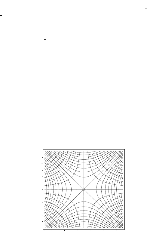
The contourplot command, with 19 contours and a 60 × 60 grid, is used to plot

φ(x, y)andψ(x, y). The plot is colored by including the option filled=true

and boxed axes are chosen. The resulting picture is shown in Figure 5.1.

contourplot({phi(x,y),psi(x,y)},x=-8..4,y=-5..7,

scaling=constrained,contours=19,grid=[60,60],

filled=true,axes=box,tickmarks=[3,3]);

–5

Figure 5.1: Streamlines and equipotentials.

The rectangular hyperboli in each quadrant are the streamlines and the curves

intersecting them at apparently 90

◦

are the equipotentials. Considering, say,

the upper-right quarter of the ﬁgure, the streamlines could represent ﬂuid ﬂow

directions near the corner of two planar surfaces intersecting at right angles.

If, say φ(x, y) = constant, then dφ =(∂φ/∂x) dx +(∂φ/∂y) dy =0, so the

slope of these curves is given by dy/dx = −(∂φ/∂x)/(∂φ/∂y). The slope of the

190 CHAPTER 5. COMPLEX VARIABLES

constant φ curves is calculated at an arbitrary point (x, y).

slope[phi]:=-diff(phi(x,y),x)/diff(phi(x,y),y);

slope

:= −

2 x +4

−2 y +2

The slope of the constant ψ curves is similarly determined.

slope[Psi]:=-diff(psi(x,y),x)/diff(psi(x,y),y);

slope

:= −

2 y − 2

2 x +4

The product of the two slopes is calculated and found to be equal to −1, so the

two sets of curves are orthogonal.

slope_product:=simplify(slope[phi]*slope[Psi]);

slope

product := −1

The complex function f = φ(x, y)+iψ(x, y) is entered, the forms of φ and ψ

being automatically entered. It is desired to express f entirely in terms of z.

f:=phi(x,y)+I*psi(x,y);

f := x

+4x − y

+2y +(2yx+4y − 2 x) I

Now, x=(z + z



)/2andy =(z −z



)/(2i), where z



is the complex conjugate of

z. These forms are substituted into f. In the output, the symbol

z represents

the conjugate of z.

f:=subs({x=(z+conjugate(z))/2,y=(z-conjugate(z))/(2*I)},f);

f := (

+2z +2z +

(z −

− (z −z) I

+(−(z −

z)(

z) I − 2 I (z −z) − z −

z) I

On applying the simplify command, f is expressed completely in terms of z.

f:=simplify(f);

f := z

+4z − 2 Iz

So, f(z)=z

+4z − 2 iz, completing the solution of the problem.

5.2 Contour Integrals

If f(z) is regular within and on a simple closed curve C, the Cauchy–Riemann

conditions lead to Cauchy’s theorem,

f(z) dz =0. (5.3)

Equivalently,



f(z) dz has a value independent of the path joining two points

and z

.Ifz

is any point inside C, Cauchy’s theorem may be used in turn

to derive Cauchy’s integral formula,

f(z)

(z − z

)

dz =2πif(z

), (5.4)

5.2. CONTOUR INTEGRALS 191

where C is traversed in a counter-clockwise direction. Note that the integrand

is not analytic at z = z

. This point is called a ﬁrst order pole or a simple pole

of the integrand. It is an example of an isolated singularity.

Cauchy’s formula may be diﬀerentiated n − 1 times to yield

f(z)

(z − z

)

dz =

2 πi

(n − 1)!



n−1

f(z)

n−1



z = z

, (5.5)

or, on setting g(z) ≡ f(z)/(z − z

)

g(z) dz =

2 πi

(n − 1)!



n−1

[(z − z

)

g(z)]

n−1



z = z

. (5.6)

The isolated singularity in g(z) is called an nth order pole, while the coeﬃcient

of 2 πi on the rhs of (5.6) is referred to as the residue of g(z)atz =z

The above formulas may be used to prove Cauchy’s residue theorem:Ifg(z)

is regular within and on the closed contour C, except for a ﬁnite number of

poles, then



g(z) dz =2πi ×(Sum of the residues of g(z)atitspoleswithinC).

5.2.1 Jennifer Tests Cauchy’s Theorem

The test of a real comedian is whether you laugh at him

before he opens his mouth.

George Jean Nathan, American critic, (1882–1958)

As a follow up to her earlier quiz, Jennifer has asked her complex variables class

to conﬁrm that Cauchy’s theorem is satisﬁed for the regular complex function

f(z = x + iy= re

iθ

)=z

− 5cos

z for the following two closed contours C:

(a) C

: (i) along the x-axis from the origin to x = 1, (ii) vertically upwards

along x =1 to y = 1, (iii) along y =1 from x =1 to x = 0, (iv) vertically

downwards along x=0 from y = 1 back to the origin;

(b) C

: (i) radially outwards along the x-axis from the origin to radius r =R,

(ii) along a circular arc of radius R from the x-axis to the y-axis,

(iii) radially inwards along the y-axis from R to the origin.

Again, Ms. Curious has been asked to present and discuss the recipe which she

has created to solve this problem.

“In (a), C

is such that rectangular coordinates should be used. Letting

f = u + iv, the general line integral is



f(z) dz =



(u + iv)(dx + idy)=



(udx− vdy)+i



(vdx+ udy). Assuming that x and y are real, f is entered

along with z =x + iy.”

restart: assume(x::real,y::real):

f:=zˆ2*exp(zˆ2)-5*cos(z)ˆ3; z:=x+I*y:

f := z

)

− 5 cos(z)

192 CHAPTER 5. COMPLEX VARIABLES

“The real and imaginary parts of f are determined (output suppressed here).”

u:=Re(f); v:=Im(f);

“For the ﬁrst leg, the integral is I1 =



(u+iv) dx, with the integrand evaluated

at y = 0. The answer is expressed in terms of the error function (erf).”

I1:=int(eval(u+I*v,y=0),x=0..1);

I1 :=

e +

√

π erf(I) −

cos(1)

sin(1) −

sin(1)

“For the second leg, the integral is I2 =



(−v + iu) dy,withx=1.”

I2:= int(eval(-v+I*u,x=1),y=0..1);

I2 := −

(−90 sin(1) e

(3 I)

− 10 sin(3) e

(3 I)

+12e

(1+3 I)

+6I

√

π erf(I) e

(3 I)

− 12 Ie

(5 I)

− 12 e

(5 I)

+6I

√

π erf(1 − I) e

(3 I)

+5Ie

+45Ie

(1+2 I)

− 5 Ie

(−3+6 I)

− 45 Ie

(−1+4 I)

(−3 I)

“For the third leg, the integral is I3 =



(u + iv) dx,withy =1.”

I3:= int(eval(u+I*v,y=1),x=1..0);

I3 :=

(5 Ie

(−3+3 I)

− 45 Ie

(1+3 I)

+57Ie

(−1+3 I)

− 6 I

√

π erf(1) e

(3 I)

− 5 Ie

(3+3 I)

− 12 Ie

(5 I)

− 12 e

(5 I)

+6I

√

π erf(1 − I) e

(3 I)

+5Ie

+45Ie

(1+2 I)

− 5 Ie

(−3+6 I)

− 45 Ie

(−1+4 I)

(−3 I)

“For the fourth leg, the integral is I4 =



(−v + iu) dy,withx=0.”

I4:=int(eval(-v+I*u,x=0),y=1..0);

I4 := −

(−3)

Ie−

(−1)

√

π erf(1) +

“Adding the four integrals and simplifying the complete contour integral CI ”

CI:=simplify(I1+I2+I3+I4);

CI := 0

“yields 0, thus conﬁrming Cauchy’s theorem. To deal with part (b), I will

unassign the Cartesian form of z, by enclosing z in right quotes, and enter its

polar form, z = re

iθ

. The complex function f then is as follows.”

z:=’z’: z:=r*exp(I*theta): f:=f;

f := r

(θI)

)

(θI)

)

− 5 cos(re

(θI)

)

“For the ﬁrst leg of the new contour C

, f is evaluated at θ = 0 and integrated

from r =0 to R.”

I1b:=int(eval(f,theta=0),r=0..R);

I1b :=

)

R +

√

π erf(RI) −

cos(R)

sin(R) −

sin(R)

“For the second leg, the integral is of the form



f(z) dz =



π/2

f(Re

iθ

) iRe

iθ

dθ.

This integration is carried out in I2b.”

5.2. CONTOUR INTEGRALS 193

I2b:=int(eval(f*I*z,r=R),theta=0..Pi/2);

I2b :=

(−6 e

(2 R

)

R − 3 I

√

π erf(RI) e

)

+ 20 cos(R)

sin(R) e

)

+40sin(R) e

)

+6IR−3 I

√

π erf(R) e

)

− 20 I cosh(R)

sinh(R) e

)

− 40 I sinh(R) e

)

(−R

)

“The third leg is radially inwards along the y axis, for which θ = π/2. The

relevant integral is performed in I3b.”

I3b:=int(eval(f*z/r,theta=Pi/2),r=R..0);

I3b :=

−1

I(6 R − 3

√

π erf(R) e

)

− 20 cosh(R)

sinh(R) e

)

− 40 sinh(R) e

)

(−R

)

“Adding the three integrals and simplifying, the complete contour integral CIb”

CIb:=simplify(I1b+I2b+I3b);

CIb := 0

“is zero, once again conﬁrming Cauchy’s theorem.”

5.2.2 Cauchy’s Residue Theorem

To know yet to think that one does not know is best;

Not to know yet to think that one knows will lead to diﬃculty.

Lao–Tzu, Chinese philosopher, 6th century BC

As a follow-up quiz to that posed in the last recipe, here’s one provided by

Jennifer for which the integrands of the contour integrals contain isolated sin-

gularities, resulting in non-zero values for the integrals. The contours are to be

traversed in a counterclockwise sense

(a) Evaluate



(5 z

−3 z

+2)/(z −1)

,withn =2, 3, 4, 5, where C is any

simple closed curve enclosing z =1. Identify the types of singularities.

(b) Evaluate



(2 z

+ z)/((z

− 1/4)(z

+2z + 2)), where the contour C is

given by (i) |z|=3/2, (ii) |z|=5/8. Identify the singular points and make

a plot showing their locations in the z-plane and the two contours.

The plottools library package is needed to plot the contours in part (b).

restart: with(plots): with(plottools):

Now, let’s tackle part (a). An operator g is introduced for generating the given

integrand (5 z

−3 z

+2)/(z −1)

for diﬀerent input values of n. Clearly, since

the numerator remains ﬁnite there, the integrand has second, third, fourth and

ﬁfth order poles at z =1 for n=2, 3, 4, 5, respectively.

g:=n->(5*zˆ4-3*zˆ2+2)/(z-1)ˆn;

g := n →

5 z

− 3 z

(z − 1)

194 CHAPTER 5. COMPLEX VARIABLES

A second operator F is formed for evaluating the integral for the nth order pole

using the Cauchy integral result in Equation (5.5).

F:=n->2*Pi*I*eval(diff(numer(g(n)),z$(n-1)),z=1)/(n-1)!;

F := n →

2 Iπ(

n−1

numer(g(n)))

z =1

(n − 1)!

Making use of F , the contour integral is evaluated for n =2, ..., 5, the results

being displayed in II(2), ..., II(5).

seq(II(n)=F(n),n=2..5);

II(2) = 28 Iπ, II(3) = 54 Iπ, II(4) = 40 Iπ, II(5) = 10 Iπ

An even easier approach to evaluating the contour integrals is to use the residue

command. An operator G is created to evaluate the residue of g(n)atz =1

and multiply the result by 2 πi.

G:=n->2*Pi*I*residue(g(n),z=1);

G := n → 2 Iπresidue(g(n),z=1)

As a check, G(n) is calculated for n=2 to 5, the answers given for II(2) to II(5)

being the same as obtained above.

check:=seq(II(n)=G(n),n=2..5);

check := II(2) = 28 Iπ, II(3) = 54 Iπ, II(4) = 40 Iπ, II(5) = 10 Iπ

The integrand for part (b) is now entered in g2 .

g2:=(2*zˆ3+z)/((zˆ2-1/4)*(zˆ2+2*z+2));

g2 :=

2 z

+ z

−

)(z

+2z +2)

One approach to evaluating the contour integral is to ﬁrst convert g2 to a

partial fraction form in terms of z.Thecomplex option allows a complete

decomposition (in ﬂoating point form) in terms of the complex roots.

g2b:=convert(g2,parfrac,z,complex);

g2b :=

0.5846153848 − 1.323076923 I

z +1. +1.000000000 I

0.6000000002

z +0.5000000000

0.5846153848 + 1.323076923 I

z +1. − 1.000000000 I

0.2307692307

z − 0.5000000000

g2b can be converted to a somewhat more compact rational form.

g2c:=convert(g2b,rational);

g2c :=

−

z +1+I

5(z +

)

z +1− I

13 (z −

)

Examining g2c, the integrand g2 has four ﬁrst order (simple) poles located at

z =1/2, −1/2, −1+i and −1 − i. Using the pointplot command, the four

simple poles are plotted as size 16 blue circles in the complex z-plane in pp.

5.2. CONTOUR INTEGRALS 195

pp:=pointplot([[1/2,0],[-1/2,0],[-1,1],[-1,-1]],

symbol=circle,symbolsize=16,color=blue):

The speciﬁed contours |z|=5/8and|z|=3/2 are circles centered on the origin

of radii 5/8and3/2, respectively. These circles are created in c1 and c2,the

smaller circle being colored red, the larger one colored green.

c1:=circle([0,0],5/8,color=red,thickness=2):

c2:=circle([0,0],3/2,color=green,thickness=2):

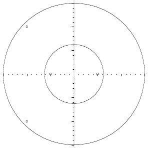
The three graphs, pp, c1,andc2, are superimposed with the display command,

the resulting picture being shown in Figure 5.2. The larger circular contour

encloses all four poles, the smaller circle enclosing only the poles at z =±1/2.

display({pp,c1,c2},labels=["x","y"]);

–1

–1 1

Figure 5.2: Four simple poles of g2 and two circular contours.

Cauchy’s residue theorem states that the contour integral is equal to 2πi times

the sum of the residues of the poles enclosed by the contour. Let’s ﬁrst consider

the contour |z|=3/2, which encloses all 4 poles. In g2c, this means that one

simply has to add the numerators of all 4 terms. The numerator of the ith term

in g2c can be extracted with the operand command op[i,1]. The 4 numerators

are then added and multiplied by2πi, yielding the answer 4πi for the integral.

I2:=2*Pi*I*add(op([i,1],g2c),i=1..4);

I2 := 4 Iπ

As shown in check2 , the same answer follows on applying the residue command

directly to g2 at each pole, adding the four residues, and multiplying by 2πi.

check2:=2*Pi*I*(residue(g2,z=1/2)+residue(g2,z=-1/2)

+residue(g2,z=-1+I)+residue(g2,z=-1-I));

check2 := 4 Iπ

Using the residue command, the value of the contour integral is now obtained

for the contour |z|=5/8 by only keeping the residues of the poles at z =±1/2.

196 CHAPTER 5. COMPLEX VARIABLES

I2b:=2*Pi*I*(residue(g2,z=1/2)+residue(g2,z=-1/2));

I2b :=

108

Iπ

In this latter case, the contour integral has the value (108/65)πi.

5.3 Deﬁnite Integrals

By performing a closed contour integration in the complex z-plane with a suit-

ably chosen path and using Cauchy’s residue theorem, it is possible to easily

evaluate some real deﬁnite integrals. The choice of path depends on the form

of the integral. A few representative examples will now be considered.

5.3.1 Inﬁnite Limits

God does not care about our mathematical diﬃculties.

He integrates empirically.

Albert Einstein, Nobel laureate in physics, (1879–1955)

To evaluate an integral of the form I =



∞

−∞

f(x) dx using contour integration,

a “standard” approach is to evaluate J =



f(z) dz with C a closed semi-

circle of radius R in the complex z-plane with its ﬂat portion along the real

axis. Along the real axis, z = x and the contribution to J is J



−R

f(x) dx.

In the limit as R →∞, J

→ I, the original integral whose value we seek.

Along the semi-circular arc, z =Re

iθ

and the line integral contribution to J is



f(Re

iθ

) iRe

iθ

dθ, if the arc is taken in the upper-half z-plane. If J

→ 0

as R →∞, evaluating J will be equivalent to evaluating I.ThevalueofJ

is then determined by calculating the sum of the residues of its poles inside C

and multiplying by 2πi. As an illustrative example, let’s evaluate the integral

I =



∞

−∞

dx/(1 + x

As suggested, we consider the contour integral J =



dz/(1 + z

)withC a

closed semi-circle of radius R in the upper-half z-plane and its ﬂat portion along

the real x-axis. The plottools library package is loaded so that the semi-circular

arc can be plotted, and the integrand of J is then entered.

restart: with(plots): with(plottools):

integrand:=1/(1+zˆ4);

integrand :=

1+z

Along the semi-circle, the line integral is J



iRe

iθ

dθ/(1 + (Re

iθ

)

). For

large R, the integrand of J

has a 1/R

dependence, so J

→ 0asR →∞.

The real axis contribution becomes the original integral. To ﬁnd its value, we

must determine the sum of the residues of any poles inside C. To this end, the

denominator of the integrand is set equal to zero and solved for the z roots.

5.3. DEFINITE INTEGRALS 197

Z:=solve(denom(integrand)=0,z);

Z :=

√

2 −

√

, −

√

−

√

2, −

√

There are four complex roots which locate four simple poles in the complex

z-plane. To see which poles contribute to the contour integral, a semi-circular

path of radius R= 2 will be drawn in the upper-half z-plane.

R:=2:

The arc command is used to draw a red semi-circle of radius R centeredonthe

origin (0,0). In the command, the angle is allowed to vary from 0 to π radians.

a:=arc([0,0],R,0..Pi,color=red,thickness=2):

The ﬂat portion of the contour between (−R, 0) and (R, 0) is plotted by entering

the end points as a list of lists and choosing a line style.

b:=plot([[-R,0],[R,0]],style=line,color=red,thickness=2):

Taking the real and imaginary parts of each root and putting them into a list

of lists, the locations of the four poles are plotted as size 16 blue circles.

c:=pointplot([seq([Re(Z[i]),Im(Z[i])],i=1..4)],

symbol=circle,symbolsize=16,color=blue):

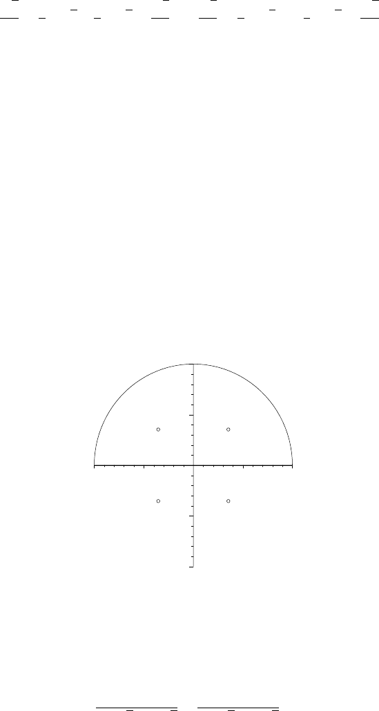
The three graphs are superimposed with constrained scaling, the resulting pic-

ture being shown in Figure 5.3.

display({a,b,c},scaling=constrained,view=[-R..R,-R..R]);

–2

–1

–2 –1 1 2

Figure 5.3: Locations of the four poles and the semi-circular contour.

Two of the poles lie inside the contour, the remaining two outside. Only the

former poles contribute to the closed contour integral. The sum r of their

residues is now calculated.

r:=residue(integrand,z=Z[1])+residue(integrand,z=Z[2]);

r :=

2 I

√

2 − 2

√

2 I

√

2+2

√