Faddeev L.D., Yakubovskii O.A. Lectures on Quantum Mechanics for Mathematics Students

Подождите немного. Документ загружается.

14 8

L. D. Faddeev and 0. A. YakubovskiT

The equation for the eigenvectors of the operator A, is

(3) A,Ei'e = ae )e

Our main assumption is that ip, and a, depend analytically oii F; that

is, they can be represented in the form

(4) a, = A(O) fi ea(1)

+62

(2)

+ .. .

(5)

V)(0)

+ F

(i) + c2V)(2) +

Substituting (4) and (5) in (3),

(A+6C)(,0(0) +eV) +

- - -) =

(A(O) +EA(l) +

.)(0(()) +e*(') +

and equating the coefficients of like powers of e, we get the system of

equations

A,o (0) = A(0)V) (0)

A,0(1) + Cv(0) =A(0)v(1) +A(1) I(0)

...............................

AV (k) + c

('-1)

= A(O) O(k) + A( 1),,(k-1) +... +

A(k),O(c}).

. . . . . . . . . . . . . . . . . . . . . . . . . . . . . . . . . . . . . .

which are more conveniently rewritten as

A'(°) =A(0)V)(0)

(s)

. . . . .

. . . .

. . .

(A A(())) V)(1) = (A(1) C)00).

\(O)) *(2) = (,\(l)

C) V(1) + \(2)V)(0),

...........................

.......................

(

_ \(O)) V)(k) = (,\(l) _ C)

(k-1) +... + A(k)V)(0)

................................................

From the first equation in (6) it fol lows31 that V)(0) is an cigenvec-

tor of A, and from the assumption about simplicity of the spectrum

we have

,1(0)

= \n,

(0)

_ 'Vn

3' Below we should equip the eigenvectors w,, the eigenvalues A, and A"), and

V M with the subscript n, but for brevity of notation we do not do that

§ 33. Perturbation theory

149

Before turning to the subsequent equations in (6) we choose a

normalization condition for the vector V),. It turns out, that the con-

dition

(7)

(V)C,,(O)) = 1

is most, convenient. We assume that ip °°) is nornialized in the usual

way: lbo) II = 1, and thus the condition (7) is equivalent to the

conditions

(8) (

{1},

{{}}) =

(,(k}. )

= o, ... .

Thus, we can look for the corrections 00),

.. ,

(k)

.... in the sub-

spawe orthogonal to the vector 0(0) = , .

Let us now consider the second equation in (6). This is an equa-

tion of the second kind with a self-adjoint operator A, and a(°) is

an eigenvalue of A. This equation has a solution if and only if the

right-hand side is orthogonal to the vector 0(0) It follows at, once

from the condition

(0(0). (A(') - C) *(())) = 0

that

V) = (C'O(())j,0(0))7

or, in more detail,

(9) ant) = (Cb, On).

The formula (9) has a very simple physical interpretation. The first-

order correction to the eigenvalue An coincides with the mean value

of the perturbation C in the unperturbed state V), n.

We consider what the second equation in (6) gives for the vector

0{1). It might seem that we should write

(10)

,(1) = (A -A(°) J)-1(a(1)

C),O(°).

However, this formula needs to be made more precise. To understand

why this is so, we consider more closely the operator (A - AI) -1,

which is called the resolvent of A. The operator A can be written in

the form

A=> AmPm,

150

L. D. Faddeev and 0. A. Yakubovskiii

where P,,, is the projection on the eigenvector 0,,; that is, P,n'p _

(Sp. ,,n } 1bm . Then for the operator (A - Al)-' we have

(11)

(A - A1)-1 =

I -

From (11) it is clear that the resolvent, loses meaning for A = an , that

is, precisely for the values of A of interest to us. However, we recall

that the right-hand side of the second equation in (6) is orthogonal to

V)(0) = Vn and ((1), p(O)) = 0. So in fact we need not the operator

(A - A])-' but the operator (A - Al) -1 P acting in the subspace

orthogonal to ion, where P is the projection I -- Pn onto that subspace.

The operator (A - A1)-1P can he represented in the form

(12)

(A-AI)1P= E

Prn

mfa

which preserves its meaning for A = An. Instead of (10) we must

write

(13)

V) (1) = (A - A (0) 1) - 1 P (A (1) - C) V) (0).

This expression can be transformed as follows-

(A - A7, I) 'P[(C n, 1Jn} bn ...' C n]

= (A - AnI)-'P(Pn - I)C

= -(A -

AnI)-' PCB'n,

and therefore

(14)

(11)

_ -(A - and) -' PCV),L

Using (12), we get that

(15)

(1) =

(Cn,'m)

An - A

rrz5n

Let us consider corrections of subsequent orders.

Froxri the or-

thogonality to

(0} of the right-hand side of the third equation in (6),

we get at once that

(16)

A(2) = (Clp(l)1 0(0)).

§ 33. Perturbation theory 151

Using the form of V)(1), we find an explicit formula for the second

correction to the eigenvalue An:

(2)

I(CV)nI

m) I2

(17)

min

An m

We shall not present the detailed computations for

,(2) and the

subsequent corrections ?,,(k) and A(k), but note only that they

can be found by the formulas A(c) = (Ci5(lt),

(O)) and 0(k)

(A -- A(°) I) -' P x [the right-hand side of the corresponding equation

in (6)].

We now discuss the theory of perturbation of a multiple eigen-

value, confining ourselves to construction of the first-approximation

correction AM. Let An = A (we omit the index n) be an eigenvalue

of A of multiplicity q:

A i = AV)i i=1,2,...,q.

Denote by N. the eigenspace of A corresponding to the eigenvalue A,

and by Q the projection on this subspace.

We turn again to the system of equations (5). As earlier, it fol-

lows from the first equation that a(°) = A. As for the vectors 00),

we can only assert that 0(0) E NA. We now show that additional

restrictions are imposed on the vectors (°), and therefore they do

not coincide with the eigenvectors Oi in the general case. Indeed, the

second equation in (6) has solutions if its right-hand side is orthogonal

to the subspace NA,; that is,

Q(A(1) - C)0(0) = 0.

Taking into account that Q*(O) = V)(°), we can rewrite the last equa-

tion in the form

(18)

QC'Q,0(°) = A(1),00)

We see that the 0(0) are eigenvectors of the q-dimensional op-

erator QCQ, and the AM are eigenvalues of it.

In practice the

problem reduces to the diagonalization of a matrix of order q.

In-

deed, substituting 0(0) = E?j ai

i in (18) and using the fact that

152

L. D. Faddeev and 0. A. Yakubovskii

we get that

ai (Ct 1, iPj )'j

A(1)

aj V j

j i

so that

Cjiaz = a(l)aj,

where Cji = (C, V)i,

V)j) .

The matrix Jis self-adjoins. and thus

can always be reduced to diagonal form. Denote the eigenvalues of

this matrix by a j(1 ), j = 1,2.....q. To the multiple eigenvalue A

of the unperturbed operator A there correspond q eigenvalues of the

operator B = A+ C. which in the first approximation of perturbation

theory have the form A + A(') , j = 1, 2, ... , q. One usually says that

the pert urhation removes the degeneracy. Of course. the removal of

the degeneracy can turn out to be incomplete if there are duplicates

among the. numbers that is, if the operator QCQ has multiple

eigenvalues.

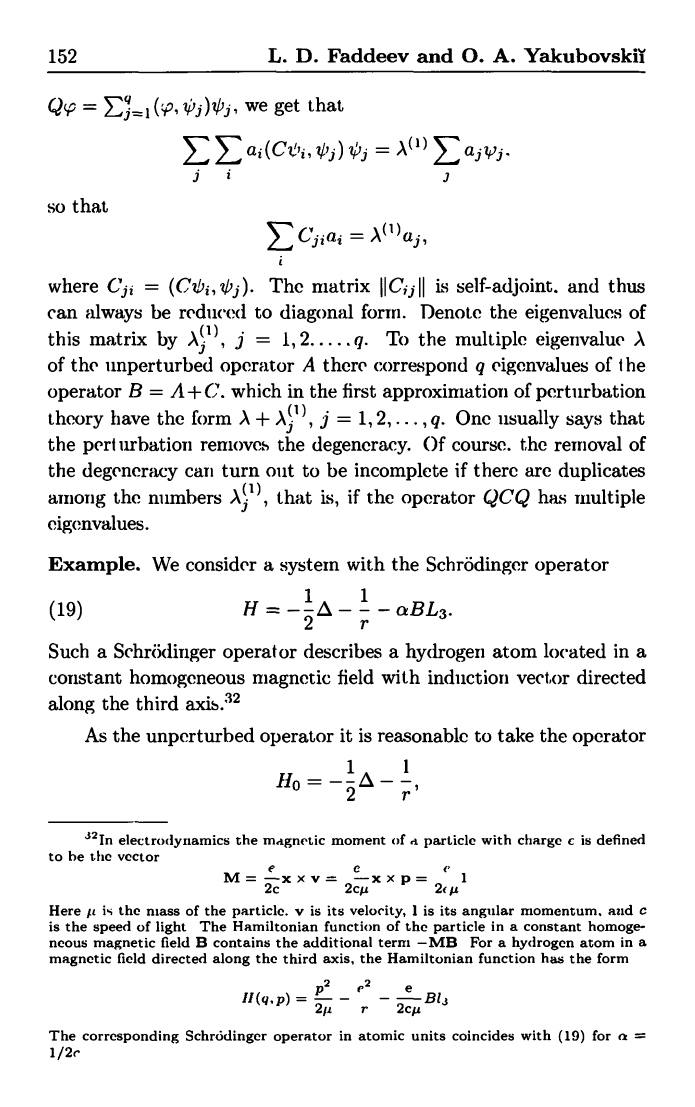
Example. We consider a system with the Schrodinger operator

H= ----aBL.

(19)

Such a Schrodinger operator describes a hydrogen atom located in a

constant homogeneous magnetic field with induction vector directed

along the third axis.32

As the unperturbed operator it is reasonable to take the operator

11_ -10-

° 2

32In electrodynamics the magnetic moment of

a particle with charge c is defined

to he the vector

P e E'

M= -XXV= 2cµxxp= 2`u1

Here is N the mass of the particle. v is its velocity, 1 is its angular momentum, and c

is the speed of light The Hamiltonian function of the particle in a constant homoge-

neous magnetic field B contains the additional term -MB For a hydrogen atom in a

magnetic field directed along the third axis, the Hamiltonian function has the form

Jf (q, p) = P2

- e2

e Bl3

2;z

r 2cM

The corresponding Schrodinger operator in atomic units coincides with (19) for n =

1/2r

§ 33. Perturbation theory

153

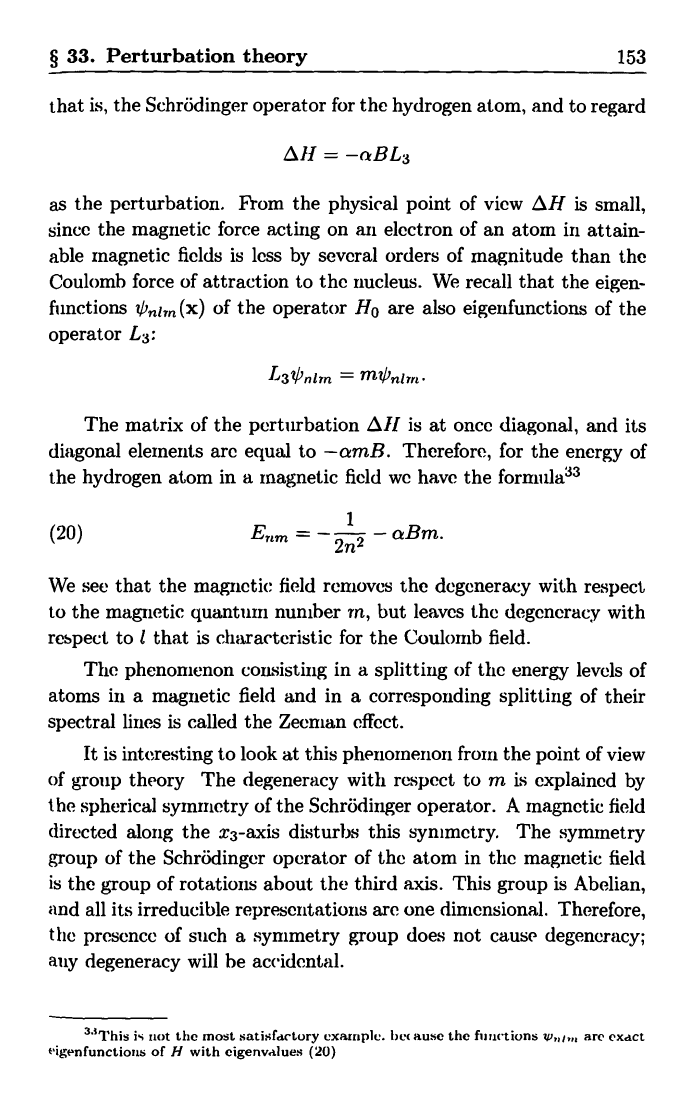
that is, the Schrodinger operator for the hydrogen atom, and to regard

Ali = -aBL3

as the perturbation. From the physical point of view

off is small,

since the magnetic force acting on an electron of an atom in attain-

able magnetic fields is less by several orders of magnitude than the

Coulomb force of attraction to the nucleus. We recall that the eigen

functions

nlrn (x) of the operator Ho are also eigenfunctions of the

operator L3:

' 3

n t rn = MOnl rn

The matrix of the perturbation MMI is at once diagonal, and its

diagonal elements are equal to --amB. Therefore, for the energy of

the hydrogen atom in a magnetic field we have the formula33

(20)

Ercm -- -`

2n2

- aBm.

We see that the magnetic field removes the degeneracy with respect

to the magnetic quantum number in, but leaves the degeneracy with

respect to l that is characteristic for the Coulomb field.

The phenomenon consisting in a splitting of the energy levels of

atoms in a magnetic field and in a corresponding splitting of their

spectral lines is called the Zeernan effect.

It is interesting to look at this phenomenon from the point of view

of group theory The degeneracy with respect to m is explained by

the spherical symmetry of the Schrodinger operator. A magnetic field

directed along the x3-axis disturbs this symmetry. The symmetry

group of the Schri;dinger operator of the atom in the magnetic field

is the group of rotations about the third axis. This group is Abelian,

aind all its irreducible representations are one dimensional. Therefore,

the presence of such a symmetry group does not cause degeneracy;

any degeneracy will be accidental.

3';This is not the most satisfactory example. because the fig rictions

are exact

t'igenfunctions of H with eigenvalues (20)

154

L. D. Faddeev and 0. A. Yakubovskii

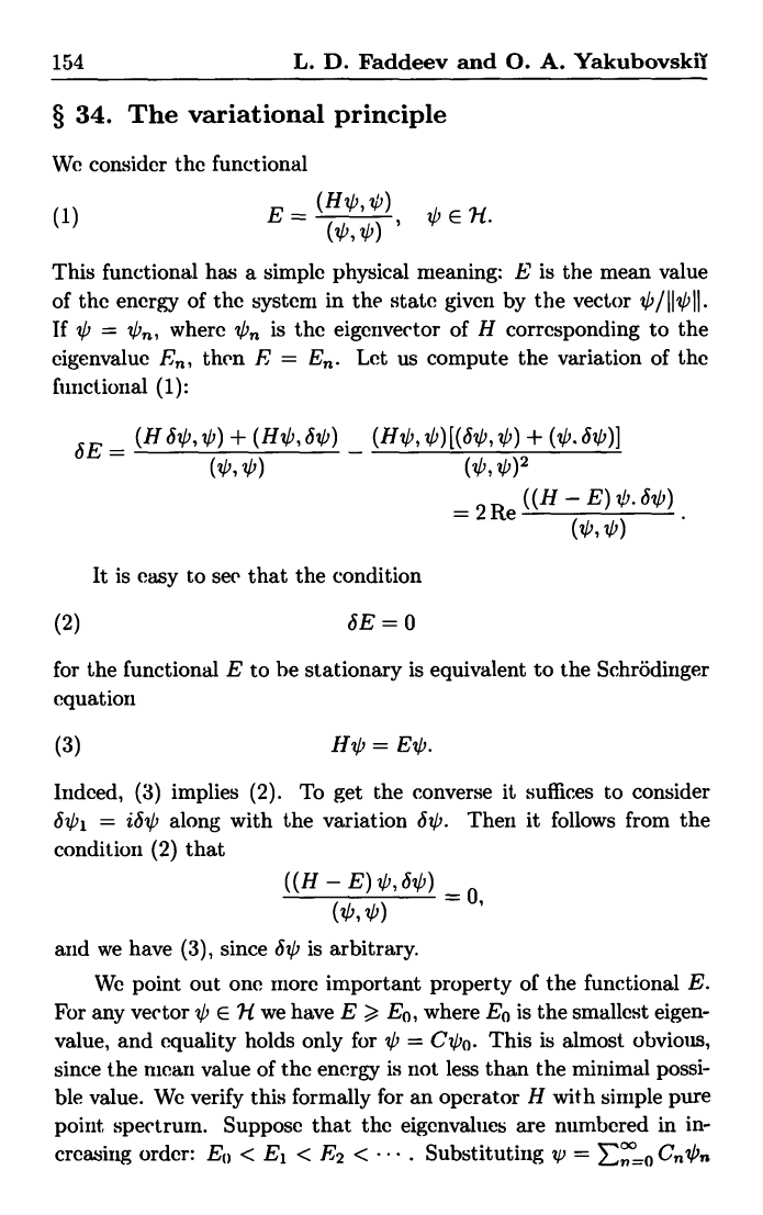
§ 34. The variational principle

We consider the functional

(HO7 0)

E l.

()

(01)

This functional has a simple physical meaning: E is the mean value

of the energy of the system in the state given by the vector V5111,011.

If 0 = , where V)n is the eigenvector of H corresponding to the

eigenvalue E, then E = E, Let us compute the variation of the

functional (1):

6E= I

(H6*jV))+(HV)j6V))

2Re

((H

E) V).

(V)I 1P)

(V)I V)) 2

It is easy to see that the condition

(2)

SE = 0

for the functional E to he stationary is equivalent to the Schrodinger

equation

(3) = Ei.

Indeed, (3) implies (2). To get the converse it suffices to consider

b*i = ibi

along with the variation &P. Then it follows from the

condition (2) that

((HE)

,60)-o,

(&,p)

and we have (3), since 60 is arbitrary.

We point out one more important property of the functional E.

For any vector 0 E' we have E > E0, where EO is the smallest eigen-

value, and equality holds only for 0 = Ci0. This is almost obvious,

since the mean value of the energy is not less than the minimal possi-

ble value. We verify this formally for an operator H with simple pure

point spectrum. Suppose that the eigenvalues are numbered in in-

CnOn

creasing order: E0 < En < F2 <

Substituting v = En=O

§ 34. The variational principle

155

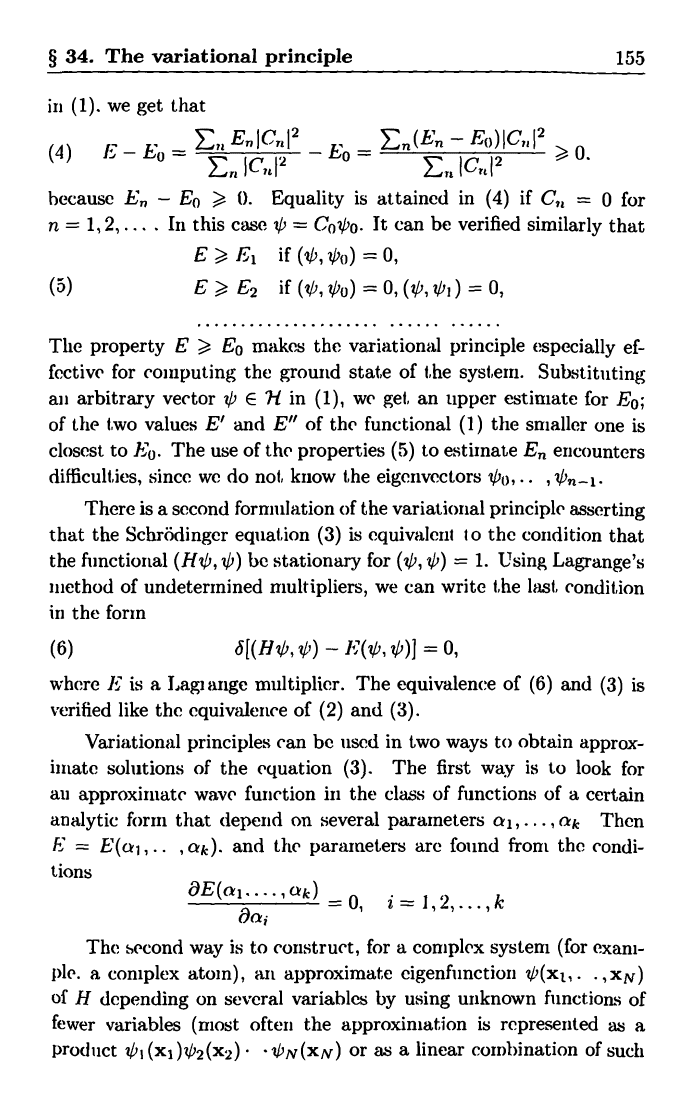
in (1). we get that

1 - E =

1:71

E IC

- E _

En (En

- Eo) iCr1

(4)

C 2

E rt

I C 2

because E,, -- Eo > 0. Equality is attained in (4) if C,, = 0 for

n = 1, 2, .... In this case ip = CoPo. It can be verified similarly that

E > E1.

,c)

(5)

E> E 2

if (V5,io)

=0,(,L,01) = 0,

..................... ...... ......

The property E > Eo makes the variational principle especially ef-

fective for computing the ground state of the system. Substituting

an arbitrary vector / E 1-1 in (1), we get, an upper estimate for E0;

of the two values E' and E" of the functional (1) the smaller one is

closest to E0. The use of the properties (5) to estimate En encounters

difficulties, since we do not know the eigenvectors

oo, ..

, iPz _ x .

There is a second formulation of the variational principle asserting

that the Schrddinger equation (3) is equivalent to the condition that

the functional (Hit',

) be stationary for (,0, 0) = 1. Using Lagrange's

method of undetermined multipliers, we can write the last, condition

in the form

(6)

a[(H, ?) ---1;(x,')1= 0,

where E is a Lagr ange multiplier. The equivalence of (6) and (3) is

verified like the equivalence of (2) and (3).

Variational principles can be used in two ways to obtain approx

inmate solutions of the equation (3).

The first way is to look for

at, approximate wave function in the class of functions of a certain

analytic form that depend on several parameters a1, ... , ak Then

E = E(a1, .. ,

ak). and the parameters are found from the condi-

tions

aE(a,....,ak)

c9cxi

The second way is to construct, for a complex system (for exam-

ple. a complex atom), an approximate eigenfiinction i'(xt,.

. , xN)

of H depending on several variables by using unknown functions of

fewer variables (most often the approximation is represented as a

product VG 1 (x1) '2 (x2) N (XN) or as a linear combination of such

156 L. D. Faddeev and 0. A. Yakubovskil

products). Equations for the functions Zi'1, .... ON are found from the

variational principle. We shall become familiar with this way when

we study complex atoms.

Example. Let us use the variational principle for an approximate

computation of the ground state of a helium atom. The Schrodinger

operator for helium in atomic units has the form

H--1Q

1Q 2 2

2 2 r1

r12

As a test function we take34

are crr2

V)(X

x2, a = e e

Computations which we omit give a simple expression for the func-

tional

E(a) = a2 --

The minimum of this expression is attained for cc = 27/16, and the

approximate theoretical value of the energy of the ground state is

E0 = E(27/16) = -(27/16)2

-2.85.

The experimental value is Ec eXp = -2.90. We see that such a sim-

ple computation leads to very good agreement with experiment. As

would be expected, the theoretical value. is greater than the experi-

mental value.

We remark that e-°r is an eigenfunction of the ground state

of a particle in a Coulomb field -a/r. Therefore, the approximate

eigenfunct ion a -270 t tr2) / 1 H is an exact eigenfunction for the operator

11,1Q -1Q 27

2 1 2

l6r1

16r2

The interaction between the electrons is taken into account in the

approximate Schrc dinger operator H' by replacing the charge Z = 2

of the nucleus by Z' = 27/16, and by the same token the screening of

the nucleus by the electron charge is taken into account.

'This choice of a test function can be ccxpl.tined by the fact that the function

27,j.-2r2 is an exact eigerufunction of the operator H

- 1 /r12

Indeed, if the term

1/r12 is removed from H, then by separation of variables the problem can be reduced

to the problem of a hydrogen-like ion, and, as has been shown, the eigenfunc tion of

the ground state of such an ion is e f' , where Z is the charge of the nucleus

§ 35. Scattering theory. Physical formulation

157

In conclusion we remark that the computations of the helium

atom used test functions with a huge number of parameters, and the

accuracy attained was such that the existing deviations from exper-

inient can be explained by relativistic corrections. Such an accurate

solution of the problem of the ground state of the helium atone has

had fundamental significance for quantum mechanics and confirms

the validity of its equations for the three-body problem.

§ 35. Scattering theory. Physical formulation of

the problem

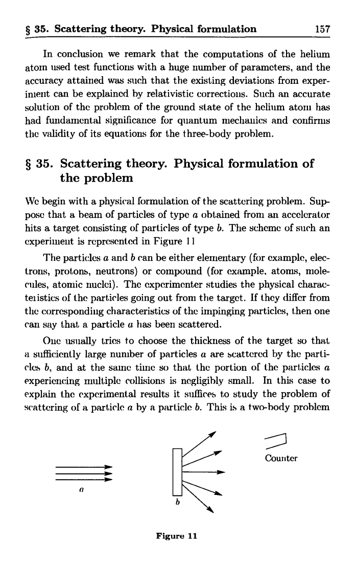
We begin with a physical formulation of the scattering problem. Sup-

pose that a beam of particles of type a obtained from an accelerator

hits a target consisting of particles of type b. The scheme of such an

experiment is represented in Figure 11

The particles a and b can be either elementary (for example, elec-

trons, protons, neutrons) or compound (for example, atoms, mole-

cules, atomic nuclei). The experimenter studies the physical charac-

tei istics of the particles going out from the target. If they differ from

the corresponding characteristics of the impinging particles, then one

can say that, a particle a has been scattered.

One usually tries to choose the thickness of the target so that

a sufficiently large number of particles a are scattered by the parti-

cles b, and at the same time, so that the portion of the particles a

experiencing multiple collisions is negligibly small.

In this case to

explain the experimental results it suffices to study the problem of

scattering of a particle a by a particle b. This is a two-body problem

Counter

am-

Figure 11