Francoise J.-P., Naber G.L., Tsun T.S. (editors) Encyclopedia of Mathematical Physics
Подождите немного. Документ загружается.


Hence, under the natural norm give n by
kf k
UðTÞ
¼ sup jS
N
ðf ; tÞj: N 2 N ¼f0; 1; ...g
f
and t 2½; g
the space U(T) is a Banach space.
We shall prove:
Theorem 1 (Kaufman 1974). Let h be a homeo-
morphism of the circle of class C
, with 3.
Suppose that
jh
00
ðtÞj þ jh
ð3Þ
ðtÞjþþjh
ðÞ
ðtÞj 6¼ 0; for all t 2 R
Then, h transports A(T) into U(T), that is, f h 2
U(T), whenever f 2A(T).
It follows from the theorem that an analytic
homeomorphism of the circle transports A(T) into
U(T). To see this, suppose that h is not of finite type.
Then, for each n 3, there exists t
n
2 [, ] such
that h
(j)
(t
n
) = 0 for all j 2 {2, ..., n}. Since {t
n
} has a
convergent subsequence, there exists t 2 [, ]
such that h
(j)
(t) = 0 for all j 2. This implies that
h
00
must be a constant function and, therefore,
h(t) = t þ . Since we know that this kind of
homeomorphism preserves A(T), we are done.
One can ask why to demand 3. The answer is
easy. Since h(t þ 2) = h(t) 2 for all t 2 R,it
follows that h
0
(t þ 2) = h
0
(t) for all t 2 R, that is, h
0
is a periodic function of period 2. So, it will always
exist a point t 2 (, ) such that h
00
(t) = 0.
We can also infer from the theorem that a C
1
homeomorphism of the circle that has no flat point,
that is, no point t such that h
(j)
(t) = 0 for all j 2,
transports A(T) into U(T). This is obvious, because
the negation of being of finite type implies the
existence of a flat point. It is not true, however, that
every C
1
homeomorphism of the circle transports
A(T) into U(T).
The proof of the theorem is based on the two
lemmas that follows. The first lemma was obtained
by Stein and Wainger, who proved it in a more
general setting in 1965, although that proof was
only published five years later. The second lemma
was proved by R Kaufman in 1974.
Lemma 2 (Stein and Wainger 1970). Let p(t) be a
real polynomial of degree d. Then
Z
r
r
e
ipðtÞ
dt
t
6ð2
dþ1
Þ2d 10
¼ 2d þ 2
X
d
k¼0
½3ð2
k
Þ2
for all r > 0.
Lemma 3 (Kaufman 1974). Let f be a real function
of class C
k
on the interval [r, r], with k 2.
Suppose that 1 jf
(k)
(t) jbforallt2 [r, r].
Then
Z
r
r
e
if ðtÞ
dt
t
C ðk; bÞ
where C(k, b) is a constant that depends only on k
and b.
We shall see that Lemma 3 can be proved from
Lemma 2 in a quite simple way. The proof given
by R Kaufman for Lemma 3 does not make use of
Lemma 2 at all. Also, it is not difficult to see that
Lemma 2 follows from Lemma 3, if we consider
d 2. So, they are indeed equivalent results.
Before getting into the proof of these two lemmas,
let us state a result which is the primary tool in
dealing with oscillatory integrals as those in the
lemmas.
Lemma 4 (Van der Corput lemma). Letfbereal
valued and smooth in [a, b], with 0 < a < b.
Suppose that jf
(k)
(t) j>0 for all t 2 [a, b].
Then
Z
b
a
e
if ðtÞ
dt
t
½3ð2
k
Þ2
1=k
a
holds if
(i) k 2, and
(ii) k = 1 and f
0
(t) is monotonic.
Now, let us prove the two lemmas and
Theorem 1.
Proof of Lemma 2 The proof is by induction on
the degree of the polynomial. Suppose that p(t)isa
polynomial of degree 0, that is, p(t) is a constant
function. In this case the result is trivial, since the
integral is equal to zero.
By induction, assume that the statement is true
for polynomials of degree less than or equal to d.
Let
pðtÞ¼a
dþ1
t
dþ1
þ a
d
t
d
þþa
1
t þ a
0
; a
dþ1
6¼ 0
Make the change of variables t = ja
dþ1
j
1=(dþ1)
s.
Then we have
Z
r
r
e
ipðtÞ
dt
t
¼
Z
e
iðqðtÞt
dþ1
Þ
dt
t
666 Homeomorphisms and Diffeomorphisms of the Circle

where = ja
dþ1
j
1=(dþ1)
r and q(t) is a polynomial
of degree at most equal to d. Suppose >1.
Then
Z
e
iðqðtÞt
dþ1
Þ
dt
t
Z
1
e
iðqðtÞðtÞ
dþ1
Þ
dt
t
þ
Z
1
e
iðqðtÞt
dþ1
Þ
dt
t
þ
Z
1
1
e
iðqðtÞt
dþ1
Þ
dt
t
I þ II þ III
By Van der Corput lemma, I [3(2
dþ1
) 2] and
II [3(2
dþ1
) 2], so I þ II 6(2
dþ1
) 4. Now
III
Z
1
1
e
iðqðtÞt
dþ1
Þ
e
iqðtÞ
hi
dt
t
þ
Z
1
1
e
iqðtÞ
dt
t
Z
1
1
jtj
d
dt þ 6ð2
dþ1
Þ2d 10
2 þ 6ð2
dþ1
Þ2d 10
since the degree of q(t) is at most equal to d.So
I þ II þ III
6ð2
dþ1
Þ4 þ 2 þ 6ð2
dþ1
Þ2d 10
¼ 6ð2
dþ1
Þ2ðd þ 1Þ10
On the other hand, if 1, then
Z
e
iðqðtÞt
dþ1
Þ
dt
t
Z
e
iðqðtÞt
dþ1
Þ
e
iqðtÞ
hi
dt
t
þ
Z
e
iqðtÞ
dt
t
2 þ 6ð2
dþ1
Þ2d 10
2 þ 6ð2
dþ1
Þ2d 10 þ 6ð2
dþ1
Þ4
6ð2
dþ1
Þ2ðd þ 1Þ10
and the proof is completed.
&
Proof of Lemma 3 Assume first that r > 1. Then
Z
r
r
e
if ðtÞ
dt
t
Z
r
1
e
if ðtÞ
dt
t
þ
Z
r
1
e
if ðtÞ
dt
t
þ
Z
1
1
e
if ðtÞ
dt
t
¼ I þ II þ III
Since jf
(k)
(t)j1 and k 2, then by Van der
Corput lemma, I [3(2
k
) 2] and II [3(2
k
) 2].
(Note that we have to assume k 2 in order to
apply Van der Corput lemma, since we know
nothing about the monotonicity of f
0
(t).)
To evaluate III, we proceed as follo wing:
f ðtÞ¼f ð0Þþf
0
ð0Þt þþ
f
ðk1Þ
ð0Þ
ðk 1Þ!
t
k1
þ
f
ðkÞ
ð
t
t Þ
k!
t
k
¼pðtÞþf
ðkÞ
ð
t
t Þ
t
k
k!
where the number
t
depends on t and 0 <
t
< 1. So
Z
1
1
e
if ðtÞ
dt
t
Z
1
1
e
iðpðtÞþf
ðkÞ
ð
t
tÞ
t
k
k!
Þ
e
ipðtÞ
hi
dt
t
þ
Z
1
1
e
ipðtÞ
dt
t
b
2
k!
þ 6ð2
k
Þ2ðk 1Þ10
by Lemma 2, since p(t) is a polynomial of degree at
most equal to k 1.
On the other hand, if r 1, it also follows from
Lemma 2 that
Z
r
r
e
if ðtÞ
dt
t
Z
r
r
e
iðpðtÞþf
ðkÞ
ð
t
tÞ
t
k
k!
e
ipðtÞ
hi
dt
t
þ
Z
r
r
e
ipðtÞ
dt
t
b
2
k!
þ 6ð2
k
Þ2ðk 1Þ10
Hence
Z
r
r
e
if ðtÞ
dt
t
Cðk; bÞ
and we are done.
&
Proof of Theorem 1 Let h be a homeomorphism
of the circle satisfying the hypotheses of the
theorem.
We claim: there exists >0 such that, for all x 2
[, ], there is k depending on x,with2 k ,
such that jh
(k)
(t þ x)j for all t satisfying jtj.
The proof of the claim is simple: suppose that
there is no such . Then, for each n 2 N and each k
with 2 k , there exist x
n
2 [, ] and t
kn
such
that jt
nk
j1=n and j h
(k)
(t
nk
þ x
n
)j < 1=n. Taking a
subsequence if necessary, we have x
n
!x 2 [, ].
Also, t
kn
!0 when n !1 for all such k. So,
h
(k)
(t
kn
þ x
n
) !h
(k)
(x) when n !1. Since jh
(k)
(t
kn
þ
x
n
)j < 1=n, we conclude that h
(k)
(x) = 0 for all k
with 2 k , thus reaching a contradiction.
Now, let f 2A(T). So ,
P
1
1
j
^
f
n
j < 1, thus
implying that
f ðtÞ¼
X
1
1
^
f
n
e
int
¼ lim
N!1
X
N
N
^
f
n
e
int
Homeomorphisms and Diffeomorphisms of the Circle 667
Hence
f ðhðtÞÞ ¼
X
1
1
^
f
n
e
inhðtÞ
¼ lim
N !1
X
N
N
^
f
n
e
inhðtÞ
Put g
N
(t) =
P
N
n = N
^
f
n
e
inh(t)
. Since g
N
is smooth,
we have g
N
2U(T) for all N 2 N.Ifg(t) stands for
f(h(t)), then g
N
!g uniformly, since f 2A(T). Thus,
it suffices to prove that g 2U(T). This happens if
and only if S
m
(g, x) =
P
m
k = m
^
g
k
e
ikx
converges uni-
formly to g as m !1, that is, given >0, there
exists m
0
2 N such that jS
m
(g, x) g(x)j < for all
m > m
0
and x 2 [, ].
We have
jS
m
ðg; xÞgðxÞj
jg
N
ðxÞgðxÞj þ jS
m
ðg
N
; xÞg
N
ðxÞj
þjS
m
ðg
N
; xÞS
m
ðg; xÞj
for all m, n 2 N.Sinceg
N
!g uniformly and g
N
2
U(T), the last inequality shows that we need to
demonstrate that, for each >0, there exists
N
0
2 N such that
S
m
ðg
N
; xÞS
m
ðg; xÞ
jj
<
8 N > N
0
; x 2½; and m 2 N
thus proving that S
m
(g
N
, x) !S
m
(g, x) uniformly in x
and m when N !1.
But, if K > N 2 N, we have
S
m
ðg
N
; xÞS
m
ðg
K
; xÞ
jj
¼
1
2
Z
g
N
ðt þ xÞg
K
ðt þ xÞðÞD
m
ðtÞdt
¼
1
2
Z
X
N
n¼N
^
f
n
e
inhðtþxÞ
X
K
n¼K
^
f
n
e
inhðtþxÞ
!
D
m
ðtÞdt
1
2
Z
X
KjnjN
^
f
n
e
inhðtþxÞ
!
D
m
ðtÞdt
1
2
X
KjnjN
j
^
f
n
j
Z
e
inhðtþxÞ
D
m
ðtÞdt
where
D
m
ðtÞ¼
X
m
k¼m
e
ikt
¼
sinðm þð1=2ÞÞt
sinðt=2Þ
is the Dirichlet kernel.
Hence, we are done if we show that
Z
e
inhðtþxÞ
D
m
ðtÞ
C ½1
where C is a constant that does not depend on m, n,
and x.
To prove that the oscillatory integral above is
bounded, we make use of Lemma 3. We have that
D
m
ðtÞ¼
2 sinðmtÞ
t
þ Oð1Þ
on any compact subset of (2,2), that is,
sinðm þð1=2ÞÞt
sinðt=2Þ
2 sinðmtÞ
t
t cosðt=2Þ2 sinðt=2Þ
t sinðt=2Þ
þ 1 C
where the constant C
does not depend on m,on
any compact subset of (2,2).
In order to prove [1], consi der x 2 [, ]. We
have already proved that there exists k (dependi ng
on x), with 2 k , such that jh
(k)
(t þ x)j>0
for all t such that jtj. The refore,
Z
e
inhðtþxÞ
sinðmt Þ
t
dt
Z
e
inhðtþxÞ
sinðmtÞ
t
dt
þ 2 log
We can assume that n is a positive integer: if n is
negative, we take complex conjugate; and if n = 0,
the integral is trivially bounded, as we see by
integration by parts or by Van der Corput lemma.
(Indeed, we do not need to worry about n = 0, since
it is necessary to bound the integral only for large n.)
So, assum ing that n is a positive integer, we
change variables: define t = rs, where r = n
1=k
1=k
.
Since sin(mt) = (e
imt
e
imt
)=(2i), we have
Z
e
inhðtþxÞ
sinðmt Þ
t
dt
Z
e
i½nhðtþxÞþmt
dt
t
þ
Z
e
i½nhðtþxÞmt
dt
t
¼
Z
=r
=r
e
i½nhðrsþxÞþmrs
ds
s
þ
Z
=r
=r
e
i½nhðrsþxÞmrs
ds
s
Put (t) = nh(rt þ x) þ mrt and (t) = nh(rt þ x)
mrt. We have
(k)
(t) = nr
k
h
(k)
(rt þ x)and
(k)
(t) =
nr
k
h
(k)
(rt þ x). But, since nr
k
= 1=, we conclude that
ðkÞ
ðtÞ
¼
ðkÞ
ðtÞ
¼
1
h
ðkÞ
ðrt þ xÞ
1; 8t 2
r
;
r
668 Homeomorphisms and Diffeomorphisms of the Circle
Also,
ðkÞ
ðtÞ
¼
ðkÞ
ðtÞ
b
k
¼
1
max jh
ðkÞ
ðsÞj: 2 s 2
no
for all t 2 [=r, =r]. Therefore, by Lemma 3, we get
Z
=r
=r
e
iðtÞ
dt
t
Cðk; b
k
Þ
max f Cðj; b
j
Þ: 2 j g
and
Z
=r
=r
e
i ðtÞ
dt
t
Cðk; b
k
Þ
max f Cðj; b
j
Þ: 2 j g
This concludes the proof.
&
Diffeomorphisms of the Circle
In this section we s tudy the circle diffe omorph-
isms. This theory goes back to Poincare´ (1885),
who studied circ le diffeomor phisms to d ecide
when differential equations on the torus have
periodic orbits of a specified type. For this he
introduced the rotation number as an important
dynamical invariant, which later turned out to be
very fruitful in the theor y of dynamical syste ms,
and proved that a diffeomorphism with an
irrational rotation number is combinatorially
equivalent to a rotation with the same rotation
number.
Denjoy (1932) constructed examples of diffeo-
morphisms of class C
1
with irrational rotation
number having wandering intervals, in opposition
to early ideas of Poincare´. It was necessary to
assume that a diffeomorphism without periodic
points is more smooth, in fact C
2
, to prove that it
is topologically conjugate to the rotation.
The Poincare´ Rotation Number
Let
e
h : T !T be an orientation-preserving homeo-
morphism. Given such a map, there is a (nonunique)
map h : R !R, which is called a lift of
e
h, such
that
e
h p = p h, where p : R !T is covering map
p(t) = e
2it
.
A lift, h,of
e
h satisfies:
1. h is monotonically increasing, that is, h(t
1
)
h(t
2
)ift
1
< t
2
.
2. h(t þ 1) = h(t) þ 1 for all t 2 R,so(h id ) has
period 1.
3. If h
1
h
2
are two lifts of
e
h, then there is an integer
k such that h
2
(t) = h
1
(t) þ k for all t 2 R.
These conditions immediately yield the following:
the transformation h
k
:= h h is monotonically
increasing and h
k
(t þ r) = h
k
(t) þ r, t 2 R, k 2 N,
r 2 Z.
The rotation number gives an asymptotic indica-
tion (i.e., in the limit) of the average amount of
rotation of a point along an orbit. We start by
defining, for a lift h of
e
h, the number
0
ðh; tÞ¼lim
k!1
h
k
ðtÞt
k
This limit exists and does not depend on the
choice of the point t 2 R; so, we denote it by
0
(h). If h
1
h
2
are two lifts of
e
h,then
0
(h
1
, t)
0
(h
2
, t)isaninteger,so
ð
e
hÞ :¼
0
ðh; tÞmod 1
is well defined. The number (
e
h) 2 [0, 1) is called the
rotation number of
e
h, and depends continuously on
e
h. For detailed proof, see Katok and Hasselblatt
(1995) or Robinson (1999).
Theorem 5 The rotation number (
e
h) is rational if
and only if
e
h has a periodic point, this is, there exist
z
0
2 S
1
and k 2 N such that
e
h
k
(z
0
) = z
0
.
Proof Take a lift h of
e
h such that h(0) 2 [0, 1).
Suppose that (
e
h) = q=m.
If
e
h has no fixed point. Then h(t) t 2 R n Z for
all t 2 R, since h(t) t 2 Z implies that p(t)isa
point fixed for
e
h. In particular, h(t) t6= q for all
t 2R, since h id is continuous and periodic, there
exist real numbers a > 0 such that h(t) t < q a for
all t 2R. Then
h
km
ðtÞh
ðk1Þm
ðtÞ
¼ h
m
½h
ðk1Þm
ðtÞ ½h
ðk1Þm
ðtÞ
< q a; 8k 2 N
+
h
km
ðtÞt
¼fh
m
½h
ðk1Þm
ðtÞ ½h
ðk1Þm
ðtÞg
þfh
m
½h
ðk2Þm
ðtÞ ½h
ðk2Þm
ðtÞg
þfh
m
½h
ðk3Þm
ðtÞ ½h
ðk3Þm
ðtÞg þ
þfh
m
ðtÞtg < kðq aÞ
So
q
m
¼ ð
e
hÞ¼lim
k!1
h
mk
ðtÞt
mk
1
m
lim
k!1
kðq aÞ
k
¼
q a
m
proving the claim by contraposition.
Homeomorphisms and Diffeomorphisms of the Circle 669

To see the converse, assume that there exists a
periodic point t
0
2 R, that is, there are m, q 2 Z
such that h
m
(t
0
) = t
0
þ q then
h
km
ðt
0
Þ¼t
0
þ kq
) ð
e
hÞ¼lim
k!1
h
mk
ðt
0
Þt
0
mk
¼
q
m
&
Corollary 6 A homeomorphism
e
h : T !T does not
have periodic points if and only if the rotation
number (
e
h) is irrational.
Let R
be defined on T by R
(e
2it
) = e
2i(tþ)
.
This map is called a rigid rotation of angle and it
is easy to see that h
(t) = t þ is lift of R
and that
(R
) = (h
) = mod 1.
In this example we can see the connection
between the rationality of the rotation number and
the existence of a periodic orbit. Assume = m=q is
rational. Then h
q
(t) = t þ q = t þ m. Therefore,
every point is periodic wi th period q. Now, assume
that is irrational. Since h
n
(t) = t þ n for all n,
then R
has no periodic points. In this case, show
that every point in T has a dense orbit.
Now, again let
e
h : T !T be any orientation-
preserving homeomorphism.
Lemma 7 If the rotation number of
e
h is rational,
then all periodic orbits have the same period .
Proof If (
e
h) = m=q with m, q 2 Z relatively prime,
then we need to show that for any periodic point
z
0
= p(t) (where p(t) = e
2it
is a covering space
projection of T) there is a lift h of
e
h such that h(0) 2
[0, 1) for which h
q
(t) = t þ m.Ifz
0
is periodic point,
then h
r
(t) = t þ s for some r, s 2 Z and
m
q
¼ ð
e
hÞ¼lim
n!1
h
rn
ðtÞt
nr
¼ lim
ns
nr
¼
s
r
So that s = km and r = kq. Then by monotonicity of
h, we have that h
q
(t) = t þ m as claimed.
&
The Poincare´ Denjoy Theory
A homeomorphism of the circle with rational
rotation number has all its orbits asymptotic to
periodic ones and this, together with Theorem 5,
yields a complete clas sifications of the possible
asymptotic behavior when the rotation number is
rational. This motivates the study of the asymptotic
behavior of orbits of homeomorphisms with irra-
tional rotation number.
The !-limit set of a point z
0
2 T with respect to
e
h
is the set !(z
0
) = {z 2 T;
e
h
n
k
(z
0
) !z as n
k
!1, for
same sequence {n
k
}
1
k = 1
}. The -limit set (z
0
)ofan
arbitrary point z
0
2 T is defined similarly (with
n
k
!1 instead n
k
!þ1).
Any orbit of a rotation R
with irrational is
dense in T, that is, !(z
0
) = (z
0
) = T for all z
0
2 T.
Theorem 8 (Poincare´ 1885). Let
e
h : T !T be an
orientation-preserving homeomorphism with irra-
tional rotation number. Then the !-limit set is
independent of x and is either T or perfect and
nowhere dense.
The preceding pr oposition says that maps with
irrational rotation number have either all orbits
dense or all orbits asymptotic to a Cantor set.
We say that two maps f , g : T !T are topologi-
cally conjugate if there exists a homeomorphism
h : T !T such that h f = g h. This implies that
h f
n
= g
n
h for every integer n. Hence, the
conjugacy h maps orbits of f into orbits of g.Ifa
monotone map l : T !T satisfies l f = g l but is
not a necessarily homeomorphism, we only have
that inverse image of each point is either a point or a
closed interval. We say that l is a semiconjugacy
between f and g; this case l maps orbits or pack of
orbits of f into orbits of g.
Theorem 9 (Denjoy 1932). Let
e
f : T !T be an
orientation-preserving diffeomorphism of class C
2
,
with irrational rotation number ((
e
f ) = ). Then
e
fis
topologically conjugate to the rigid rotation R
.
Note that in spite of the hypothesis of
e
f being C
2
,
we obtain only a continuous conjugacy. It took
almost 50 years until Michael Herman (1979) was
able to solve the more difficult problem of obtaining
a smooth conjugacy for rotat ion number satisfying
extra arithmetic conditions.
If
e
f is a circle homeomorphism which does not
have periodic points, then there exists a semicon-
jugacy h between
e
f and a rotation R
.Ifh is not a
conjugacy, then there exists a point x of the circle
whose inverse image by h is an interv al J.Since
h
e
f = R
h,wehavethath(
~
f
n
(J)) = R
n
(x). It
follows that the intervals of the family
{ J, f ( J), f
2
( J), ...} are pairwise disjoint, and the
!-limit set of J does not reduce to a periodic orbit.
We say that J is a wandering interval of the map
e
f .
Thus, C
2
-differentiability implies that
e
f does not
have a w andering interval. For details of the proof
of Theorem 9, see MeloandStrien(1993).
The Denjoy Example
Denjoy also proved the following result, which
shows that the hypothesis of class C
2
is essential.
Theorem 10 (Denjoy 1932). For any irrational
number 2 [0, 1), there exists a C
1
-circle diffeo-
morphism f which has a wandering interval, and
rotation number equal to .
670 Homeomorphisms and Diffeomorphisms of the Circle

Proof The construction of a diffeomorphism with
wandering interval will be done in the following
manner. Given an irrational rotation R
(e
2it
) =
e
2i(tþ)
, cut the circle T at all the points of an orbit
{z
n
= R
n
(e
2it
0
); n 2 Z}ofR
. In each cut insert a
segment J
n
of length l
n
where
P
1
n = 1
l
n
= 1. We
obtain in this manner a new circle longer than the
first. The open intervals correspond to the gaps of
the Cantor set.
In order to construct f formally. Let l
n
be a
sequence of positive real numbers with n 2 Z
satisfying
(i) lim
n !1
(l
nþ1
/l
n
) = 1
(ii)
P
1
n = 1
l
n
= 1
(iii) l
n
> l
nþ1
for n 0
(iv) l
n
< l
nþ1
for n < 0 and
(v) 3l
nþ1
l
n
> 0 for n 0
For example
l
n
¼ Tðjnjþ2Þ
1
ðjnjþ3Þ
1
where
T
1
¼
X
1
n¼1
ðjnjþ2Þ
1
ðjnjþ3Þ
1
Let J
n
be a closed interval of length l
n
. We place
these intervals on the circle in the same order as the
order of the orbit R
n
(0). So to place an interval J
n
,
consider the sum of the lengths of the intervals J
i
where R
i
(0) is between R
n
(0) and 0. This deter-
mines the placement of J
n
.
The next step is to define f on the union of the J
n
.
It is necessary and sufficient for f
0
(t) = 1onthe
endpoint in order for the map to have a continuous
derivative when it is extended to the closure.
Assume J
n
= [a
n
, b
n
], so l
n
= b
n
a
n
. The integral
Z
b
n
a
n
ðb
n
tÞðt a
n
Þdt ¼
l
3
n
6
so
6ðl
nþ1
l
n
Þ
l
3
n
Z
b
n
a
n
ðb
n
tÞðt a
n
Þdt ¼ l
nþ1
l
n
Therefore, if we define f for x 2 J
n
by
f ðxÞ¼a
nþ1
þ
Z
x
a
n
1 þ
6ðl
nþ1
l
n
Þ
l
3
n
ðb
n
tÞðt a
n
Þ
dt
then f (b
n
) = a
nþ1
þ l
n
þ l
nþ1
l
n
= b
nþ1
. Also, f is
differentiable on J
n
with
f
0
ðxÞ¼1 þ
6ðl
nþ1
l
n
Þ
l
3
n
ðb
n
xÞðx a
n
Þ
Thus, f
0
(a
n
) = 1 = f
0
(b
n
). Notice that for n < 0, l
nþ1
l
n
> 0, that
1 f
0
ðxÞ1 þ
6ðl
nþ1
l
n
Þ
l
3
n
l
n
2
2
¼
3l
nþ1
l
n
2l
n
and (3l
nþ1
l
n
)=(2l
n
) goes to 1 as n !1. Simi-
larly for n 0 and x 2 J
n
,
1 f
0
ðxÞ
3l
nþ1
l
n
2l
n
> 0
so f
0
(x) goes to 1 as n !þ1uniformly for x 2 J
n
.
From these facts, it follows that f is uniformly C
1
on
the union of the interiors of the J
n
and has a C
1
extension to all of T.
Let =Tn[
n2Z
int(J
n
). This is a Cantor set. The
orbit of a point x 2 is dense in since it is like the
orbit of 0 for R
. Thus, !(x) =.Ifx 2 int(J
n
), then
there is a smaller interval I whose closure is
contained in int(J
n
). Since the inte rval J
n
never
returns to J
n
but wanders among the other J
k
, then
J
n
is a wandering interval.
&
Further Results
In this sect ion we shall state some additional results
about homeomorphisms of the circle in the area of
Fourier analysis.
The first result is a theorem of Pa´l (1914) and
Bohr (1935): let f : T !R be a real continuous
function; then, there exists a homeomorphism of the
circle h such that f h 2U(T). The best proof of this
theorem is due to Salem (1945). In 1978, Kahane
and Katznelson showed that the result is still valid
for f : T !C continuous.
A similar question was posed by Lusin: given a
continuous function f : T !R, is there a home-
omorphism of the circle h such that f h 2A(T)?
The problem remained open until 1981, when
Olevskii, Kahane, and Katznelson answered nega-
tively the question: there exists a real (or complex)
continuous function f on the circle, such that, for all
homeomorphism of the circle h, f h 62A(T).
It was proved by the author that there are C
1
homeomorphisms of the circle, not necessarily of
finite type, that transport A(T) into U(T ). It is a very
technical work, published in 1998, and it gives a
necessary and sufficient condition for a homeo-
morphism of the circle with a flat point to transport
A(T) into U(T).
Finally, the Denjoy theorem (Theorem 9) is rather
close to being optimal. The example constructed here
can be improved by obtaining a circle diffeomorphism
whose first derivatives have Ho¨ lder exponent arbitrarily
closeto1(seeKatok and Hasselblatt (1995)). Recent
Homeomorphisms and Diffeomorphisms of the Circle 671

work has dealt with the existence of a differentiable
conjugacy between a diffeomorphism f with irrational
rotation number and R
. Arnol, Moser, and Herman
have obtained results (see Melo and Strien (1993) for a
discussion of this results and references).
Acknowledgments
The author was supported in part by CNPq-
Brazil. and was partially supporte d by FAPESP
Grant # TEMA
´
TICO 03/03107-9.
See also: Chaos and Attractors; Ergodic Theory; Generic
Properties of Dynamical Systems; Random Dynamical
Systems; Wavelets: Mathematical Theory.
Further Reading
Denjoy A (1932) Sur les courves de´finies par les e´quations
differe´ntialles a la surface du tore. Journal de Mathe´matiques
Pures et Applique´es 11(9): 333–375.
Herman M (1979) Sur les conjugation diffe´rentiable des diffe´o-
morphisms du cercle a` des rotations. Publ. Math. IHES 49:
5–233.
Kahane JP (1970) Se´ries de Fourier Absolument Convergentes,
p. 84. Berlin: Springer.
Kahane JP (1983) Quatre Lec¸ ons sur les Home´omorphismes du
Circle et les Series de Fourier. In: Topics in Modern Harmonic
Analysis, Proceedings of a Seminar Held in Torino and
Milano, May–June 1982, vol. II, pp. 955–990. Roma.
Katok A and Hasselblatt B (1995) Introduction to the Modern
Theory of Dynamical Systems. Cambridge: Ca mbridge
University Press.
Katznelson Y (1976) An Introduction to Harmonic Analysis, 2nd
edn, p. 217. New York: Dover.
Melo W and Strien S (1993) One-Dimensional Dynamics, ch. 1.
Berlin: Springer.
Poincare´ H (1881) Me´moire Sur les courves de´finies par les
e´quations differe´ntialles I. Journal of Mathe´matiques Pures et
Applique´es 3(7): 375–422.
Poincare´ H (1882) Me´moire Sur les courves de´finies par les
e´quations differe´ntialles II. Journel de Math. Pure et Appl. 8:
251–286.
Poincare´ H (1885) Me´moire Sur les courves de´finies par les
e´quations differe´ntialles III. Journel de Math. Pure et Appl.
4(series 1): 167–244.
Poincare´ H (1886) Me´moire Sur les courves de´finies par les
e´quations differe´ntialles IV. Journel de Math. Pure et Appl. 2:
151–217.
Robinson C (1962) Dynamical Systems: Stability, Symbolic
Dynamicas, and Chaos. London: CRC Press.
Robinson C (1999) Dynamical Systems: Stability, Symbolic
Dynamics, and Chaos. London: CRC Press.
Rudin W (1962) Fourier Analysis on Groups, ch. 4. New York:
Wiley.
Stein EM (1986) In: Stein EM (ed.) Oscillatory Integral and
Fourier Analysis, Beijing Lectures in Harmonic Analysis,
pp. 307–355. Princeton: Princeton University Press.
Stein EM and Wainger S (1970) The estimation of an integral
arising in multiplier transformation. Studia Math. 35:
101–104.
Zumpano A (1998) Infinite type homeomorphisms of the circle
and convergence of Fourier series. Transactions of the
American Mathematical Society 350(10): 4023–4040.
Homoclinic Phenomena
S E Newhouse, Michigan State University,
E. Lansing, MI, USA
ª 2006 Elsevier Ltd. All rights reserved.
Introduction
Homoclinic orbits (or motions) were first defined by
Poincare´ in his treatise on the ‘ ‘restricted three-body
problem.’’ (Poincare´ 1987) Further advances were
made by Birkhoff (Birkhoff 1960) in the 1930s, and,
by Smale in the 1960s. Since that time, they have been
studied by many people and have been shown to be
intimately related to our understanding of nonlinear
dynamical systems. There are many systems which
possess homoclinic orbits. In one striking example (as
discussed in the book of Moser (1973),theycanbe
used to account for the unbounded oscillatory motion
discovered by Sitnikov in the three-body problem. They
also commonly occur in two-dimensional mappings
derived from periodically forced oscillations (e.g., see
the book by Guckenheimer and Holmes (1983).
Roughly speaking, a homoclinic orbit is an orbit
of a mapping or differential equation which is both
forward and backward asymptotic to a periodic
orbit which satisfies a certain nondegeneracy condi-
tion called ‘‘hyperbolicity.’’ On its own, such an
orbit is only of mild interest. However, these orbits
induce quite interesting structures among nearby
orbits, and this latter fact is responsible for the main
importance of homoclinic orbits. In addition, when
homoclinic orbits are created in a parametrized
system, many interesting and unexpected phenom-
ena arise.
In this article, we first describe the history and
basic properties of homoclinic orbits. Next, we
consider some simple polynomial diffeomorphisms
of the plane (the so-called He´non family) which
exhibit homoclinic orbits. Subsequently, we discuss
a general theorem due to Katok which gives
sufficient conditions for the existence of such
orbits. Finally, we briefly consider issues related to
homoclinic bifurcations and some of their
consequences.
672 Homoclinic Phenomena
Homoclinic Orbits in Diffeomorphisms
Consider a discrete dynamical system given by a C
r
diffeomorphism f : M !M where M is a C
1
mani-
fold and r is a positive integer. That is, f is bijective
and both f and f
1
are r-times continuously
differentiable. Given a point x 2M, set x
0
= x. For
non-negative integers n we inductively define
x
nþ1
= f (x
n
) and x
n1
= f
1
(x
n
). We also write
f
n
(x) = x
n
for n in the set Z of all integers. The
‘‘orbit’’ of x is the set O(x) = {f
n
(x): n 2Z}.
A ‘‘periodic point’’ p of f is a point such that there
is a positive integer N > 0 such that f
N
(p) = p. The
least such number (p) is called the ‘‘period’’ of p.If
(p) = 1, we call p a ‘‘fixed point.’’ The periodic
point p with period is called called ‘‘hyperbolic’’ if
all eigenvalues of the derivative Df
(p)atp have
absolute value different from 1. For convenience, we
refer to the eigenvalues of Df
(p) as eigenvalues
associated to p.Ifp is a hyperbolic periodic point all
of whose associated eigenvalues have norm less than
one, we call p a ‘‘sink’’ or ‘‘attracting periodic
point.’’ The opposite case in which all associated
eigenvalues have norm larger than one is called a
‘‘source.’’ A hyperbolic periodic point p which is
neither a source nor a sink is called a ‘‘saddle’’ or
‘‘hyperbolic saddle.’’
Given a saddle p of period , we consider the set
W
s
(p) = W
s
(p, f ) of points y 2M which are forward
asymptotic to p under the iterates f
n
. That is, the
points y 2M such that f
n
(y) !p as n !1. This is
called the ‘‘stable set’’ of p. Similarly, we consider
the ‘‘unstable set’’ of p which we may define as
W
u
(p) = W
u
(p, f ) = W
s
(p, f
1
). The stable manifold
theorem guarantees that W
s
(p)andW
u
(p) are
injectively immersed submanifolds of M whose
dimensions ad d up to dim M. In these cases, they
are called the stable and unstable manifolds of p,
respectively. A point q 2W
s
(p)
T
W
u
(p) n{p}iscalled
a ‘ ‘homoclinic point’’ of p (or of the pair (f, p)). If the
submanifolds W
s
(p)andW
u
(p)meettransverselyatq,
then q is called a ‘‘transverse homoclinic point.’’
Otherwise, q is called a ‘‘homoclinic tangency.’’
In the special case when M is a two-dimensional
manifold, the stable and unstable manifolds of a
saddle periodic point p are injectively immersed
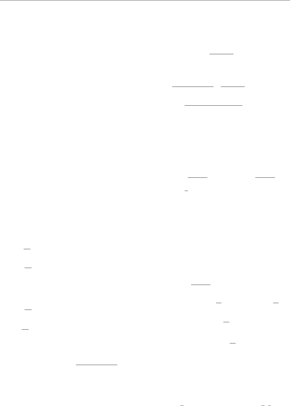
curves in M. A transverse homoclinic point q of p is
a point of intersection off p where the curves are not
tangent to each other. This is depicted in Figure 1
for the case of a saddle fixed point for the map
H(x, y) = (7x
2
y, x), a member of the so-called
He´non family, which we will discuss later. The
figure was made using the numerical package
‘‘Dynamics’’ which comes with the book by Nusse
and Yorke (1998).
One easily sees that every point in the orbit of
a transverse homoclinic point q of a hy perbolic
saddle fixed point p is again a transverse homoclinic
point of p. Also, the curves W
u
(p) and W
s
(p) are
invariant; that is, f (W
u
(p)) = W
u
(p)andf (W
s
(p)) =
W
s
(p). This implies that the curves W
u
(p) and W
s
(p)
extend, wind around, and accumulate on each other
forming a complicated web.
Upon seeing this complicated structure in the
restricted three-body problem, Poincare´ very poeti-
cally wrote (p. 389, Poincare´ 1987)
Que l’on cherche a` se repre´senter la figure forme´e par
ces deux courbes et leurs intersections en nombre infini
dont chacune correspond a` une solution doublement
asymptotique, ces intersections forment une sorte de
treillis, de tissu, de re´seau a` mailles infiniment serre´es;
chacune des deux courbes ne doit jamais se recouper
elle-meˆme, mais elle doit se replier sur elle-meˆme d’une
manie` re tre´s complexe pour venir recouper une infinite´
de fois toutes les mailles du re´seau.
On sera frappe´ de la complexite´ de cette figure, que je
ne cherche meˆme pas a` tracer. Rien n’est plus propre a`
nous donner une ide´e de la complication du proble`me
des trois corps et en ge´ne´ral de tous les proble` mes de
Dynamique ou` il n’y a pas d’inte´ grale uniforme ...
The next major advance concerning homoclinic
orbits was made by Birkhoff (1960), who proved
that in every neighborhood of a transverse
homoclinic point of a surface diffeomorphism,
one can find infinitely many distinct periodic
points. Birkhoff also presented a symbolic
description of th e nearby orbits and noticed the
analogy with Hadamard’s description of geodesics
on a surface. Birkhoff’s analysis was generalized
by Smale to arbitrary dimension, and, in addition,
Smale gave a simpler analysis of the associated
nearby orbits in terms of compact zero-dimensional
W
u
(p)
W
s
(p)
q
p
Figure 1 Stable and unstable manifolds in the map
H(x, y) = (7 x
2
y , x ) for the fixed point p (3.83, 3.83).
Homoclinic Phenomena 673
symbolic spaces which we now call ‘‘shift spaces’’
or ‘‘topological Markov chains.’’
Once one knows that a diffeomorphism f has a
transverse homoclinic point for a saddle periodic
point p, it is interesting to consider the closure of the
orbits of all such homoclinic points. This turns out
to be a closed invariant set containing a dense orbit
and a countable dense set of periodic saddle points
(Newhouse 1980). It is usually called a ‘‘homoclinic
closure’’ or h-closure. These sets form the basis of
chaotic or irregular motions in nonlinear systems.
The Smale Horseshoe Map and
Associated Symbolic System
To understand the geometric picture discovered by
Smale, it is best to start with a concrete example of a
diffeomorphism of the plane known as the ‘‘Smale
horseshoe diffeomorphism.’’
Given any homeomorphism f : X !X on a space
X and a subset U X, let us define I(f , U) to be the
set of points x 2X such that f
n
(x) 2U for every
integer n. Thus, we have
Iðf ; UÞ¼
\
n 2Z
f
n
ðUÞ
We call I(f , U) the invariant set of f in U, or,
alternatively, the invariant set of the pair (f , U).
We now construct a special diffeomorphism f of
the Euclidean plane to itself in which U = Q is the
unit square and for which I(f , U) has a very
interesting structure. It is this map which is usually
known as the Smale horseshoe map.
Let Q = [0, 1] [0, 1] be the unit square in the
plane R
2
. Let 0 <<1=2, and consider a diffeo-
morphism f : R
2
!R
2
which is a composition of two
diffeomorphisms f = T
2
T
1
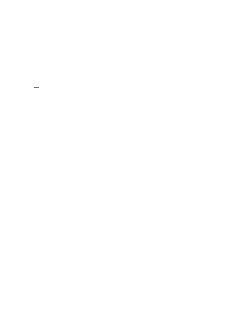
as follows. The map
T
1
(x, y) = (
1
x, y) contracts vertically, expands
horizontally, and maps Q to the thin rectangle
Q
1
= {(x, y):0 x
1
,0 y } which is short
and wide. The map T
2
bends the right side of Q
1
up
and around so that T
2
(Q
1
) = f ( Q) has the shape of a
‘‘horseshoe’’ or ‘‘rotated arch. ’’ We arrange for T
2
to
take the lower-right corner of Q
1
up to the upper-left
corner of Q in such a way that f (Q) meets Q in two
full width subrectangles which we call R
1
and R
2
.
This can be done in such a way that the preimages
R
1
1
= T
1
1
(R
1
) and R
1
2
= T
1
1
(T
1
2
(R
2
)) are both full-
height subrectangles of Q, and the restricted maps
f
1
def
=
f j R
1
1
and f
2
def
=
f j R
1
2
are both affine. Thus, we
arrange that f
1
is simply the restriction of T
1
to R
1
1
,
and the map f
2
can be expressed in formulas as
f
2
(x, y) = (
1
x þ
1
, y þ 1). This construc-
tion implies that f will have the origin p = (0, 0) as a
hyperbolic fixed point. We label the upper-left corner
(0, 1) of Q with the letter q. It follows that the bottom
and left edges of Q will be in the unstable and stable
manifolds of p, respectively, and we have indicated
this in Figure 2 with small arrows.
The above construction gives us a diffeomorphism
f of the plane R
2
such that Q
þ
1
def
=
f (Q)
T
Q =
R
1
S
R
2
is the union of two full-width subrectangles
of Q. We wish to describe I(f , Q). We begin with
the sets Q
þ
=
T
n0
f
n
(Q) and Q
=
T
n0
f
n
(Q).
Thus, Q
þ
is simply the set of points in Q whose
backward orbits stay in Q, and Q
is the set of
points whose forward orbits stay in Q. For i = 1, 2,
each rectangle R
i
is mapped to a thin horseshoe in
f (Q) which meets Q in two full-width subrectangles.
Combining these for i = 1, 2 gives four full-width
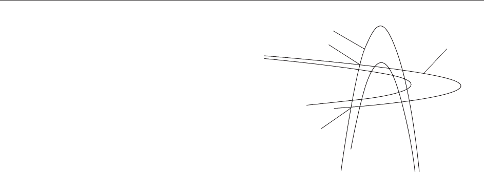
rectangles as shaded in Figure 3. Thus,
Q
T
f (Q)
T
f
2
(Q) consists of these four subrectan-
gles. Figure 3 shows the sets f
2
(Q), f
2
(Q) as well as
the shaded rectangles we just mentioned.
Continuing in this way, one sees that, for each
n > 0, the set Q
þ
n
= Q
T
f (Q)
T
...
T
f
n
(Q) consists
of 2
n
full-width subrectangles of Q, each with height
p
q
f
–2
(Q)
f
2
(Q)
Figure 3 The sets f
2
(Q) and f
2
(Q) for the horseshoe map f.
q
p
Q
f(Q)
Q
R
2
R
1
Q
1
T
1
Figure 2 The horseshoe map.
674 Homoclinic Phenomena

n
. It follows that Q
þ
=
T
n
f
n
(Q) is an inte rval
times a Cantor set. Analogously, Q
is a Cantor set
times an interval, and the set I(f , Q) is a Cantor set
in the plane. Let us recall the definition of a Cantor
set C in a metric space X. We first define a Cantor
space C to be a compact, perfect, totally discon-
nected metric space. That is, C is a compact metric
space, whose connected components are points such
that every point x in C is a limit point of C n{x}. A
Cantor set C in a metric space X is a subset which is
a Cantor space in the induced subspace (relative)
topology.
The dynamics of f on the invariant set I(f , Q ) can
be conveniently described as follows.
Let
2
= {1, 2}
Z
be the set of doubly infinite
sequences of 1’s and 2’s. Writing elements a 2
2
as a = (a
i
) = (a
i
)
i 2Z
, we define a metric on
2
by
ða; bÞ¼
X
n 2Z
1
2
jnj
ja
i
b
i
j
The pair (
2
, ), then, is a Cantor space.
The ‘‘left-shift automorphism’’ on
2
is the map
:
2
!
2
defined by (a)
i
= a
iþ1
for each i 2Z.
This is a homeom orphism from
2
to itself. It has a
dense orbit and a dense set of periodic points.
For a point x 2I(f , Q), define an element (x) =
a = (a
i
) 2
2
by a
i
= j if and only if f
i
(x) 2R
j
. It turns
out that the map : I(f , Q) !
2
is a homeomorph-
ism such that = f .
In general, given two discrete dynamical syst ems
f : X !X, and g : Y !Y, a homeomorphism
h : X !Y such that gh = hf is called a topological
conjugacy from the pair (f, X) to the pair (g, Y).
When such a conjugacy exists, the two systems have
virtually the same dynamical properties.
In the present case, one sees that the dynamics of f
on I(f , Q) is completely described by that of
on
2
.
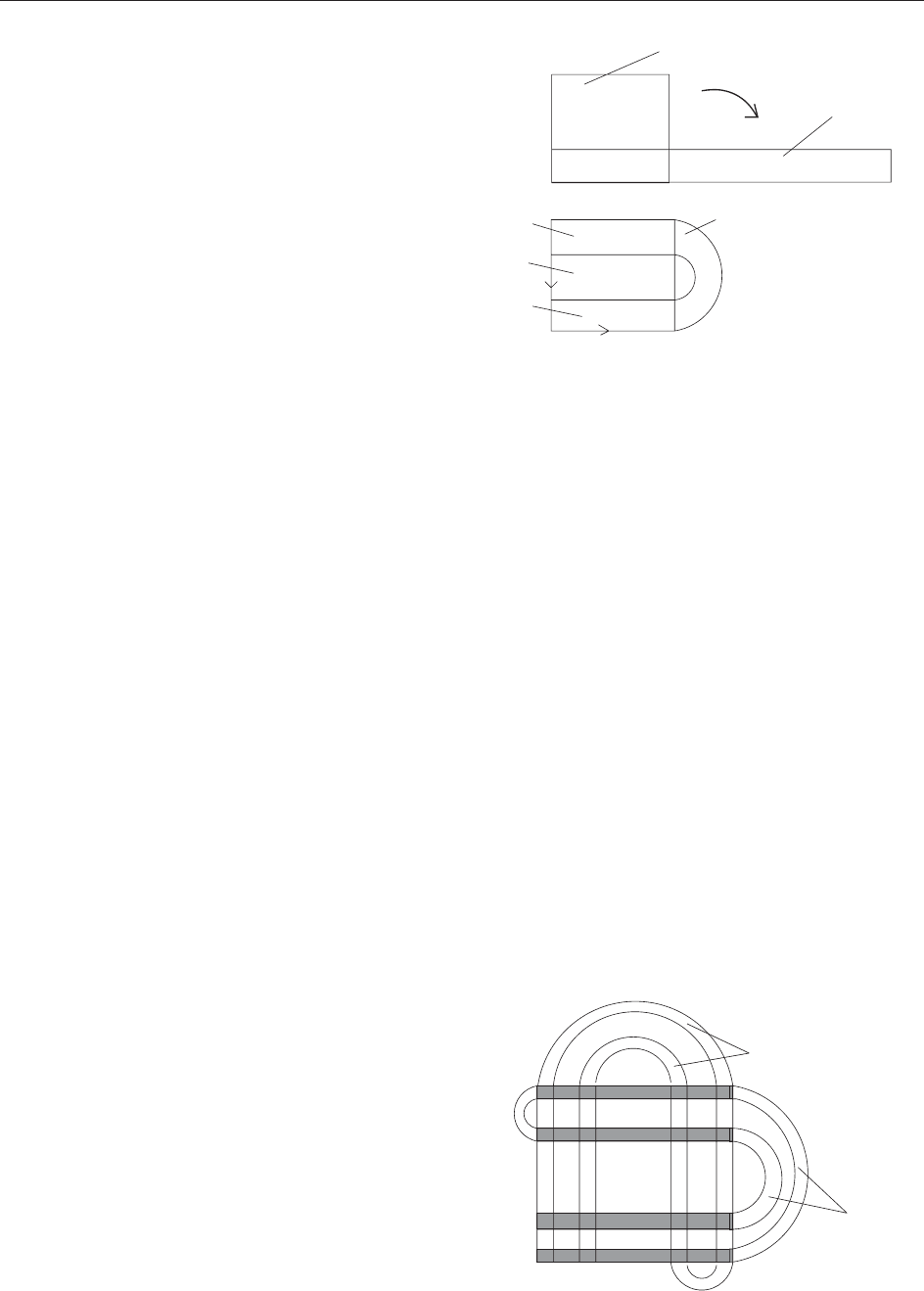
It turns out the the Smale horseshoe map contains
essentially all of the geometry necessary to describe
the orbit structures near homoclinic orbits. To begin
to see this, recall that the left and bottom boundaries
of Q were in the stable and unstable manifolds of p.
Extending these curves as in Figure 4, one sees that
the three corners of Q different from p are, in fact,
all transverse homoclinic points of p.
It was a great discovery of Smale that, in the case
of a general transverse homoclinic point, one sees
the above geometric structure after taking some
power f
N
of the diffeomorphism f. Thus, we have
Theorem 1 (Smale). Let f : M !MbeaC
1
diffeo-
morphism of a manifold M with a hyperbolic
periodic point p and a transverse ho moclinic point
q of the pair (f, p). Then, one can find a positive
integer N and a compact neighborhood U of the
points p and q such that the pair (f
N
, I(f
N
, U)) is
topologically conjugate to the full 2-shift (,
2
).
In modern language, we can assert that more
is true. Let (f ) =
S
0j<N
f
j
(I(f
N
, U)) be the f-orbit
of the set I(f
N
, U). Then, (f ) is a compact zero-
dimensional hyperbolic basic set for f with
V
def
=
S
0j<N
f
j
(U) as an ‘‘adapted’’ or ‘‘isolating’’
neighborhood. This means that (f ) =
T
n 2Z
f
n
(V)
is a compact, zero-d imensional hyperbolic set (see
Robinson (1999) for definitions and related refer-
ences) contained in the interior of V and f j (f ) has
a dense orbit. If g is C
1
near f, then
(g)
def
=
T
n 2Z
g
n
(V) is a hyperbolic basic set for g
and the pairs (f , (f )) and (g, (g)) are topologically
conjugate.
To get some appreciation for the magnitude of the
contribution here, one might note the complicated
arguments employed by Poincare´attheendof
Poincare´ (1987) to show that so-called heteroclinic
points (intersections between stable and unstable
manifolds of saddles with different orbits) existed.
Birkhoff found a symbolic description (using infinitely
many symbols) of the orbits near a transverse
homoclinic orbit from which the existence of both
infinitely many periodic and heteroclinic points is
obvious. Smale extended the treatment of transverse
homoclinic points to all dimensions, and found the
symbolic description (using two symbols for some
iterate of the map) given above. Moreover, Smale
proved the ‘ ‘robustness’’ of these structures: they persist
under small C
1
perturbations. Note that Poincare´’s
discovery of homoclinic points was in 1899, Birkhoff’s
results came in 1935, and Smale’s results came in
1965. Thus, the above advances took over 65 years!
One can understand the geometry of Smale’s
construction fairly easily in the two-dimensional
case. Let q be the transverse homoclinic point of the
saddle fixed point p of the C
r
diffeomorphism f on
the plane R
2
. Given a small neighborhood
~
U of p, let
Figure 4 Stable and unstable manifolds in the horseshoe map.
Homoclinic Phenomena 675