Francoise J.-P., Naber G.L., Tsun T.S. (editors) Encyclopedia of Mathematical Physics

Подождите немного. Документ загружается.

The Dispersive Property

Consider for the solutions in R

 R

of the

elementary kinetic equations

f þ v r

f ¼ 0; f ðx; v; 0Þ¼f

ðx; vÞ½44

the local density

ðx; tÞ¼

f ðx; v; tÞ dv ½45

From the relation

jðx; tÞj ¼

f ðx; v; tÞdv

ðx  vt; v; tÞdv



sup

w2R

ðx  vt; wÞjdv ½46

deduce with an elementary change of variable the

following estimate, which carries the name of

dispersion lemma,

jðx; tÞj 

jtj

ðR

ÞÞ

½47

From interpolation and duality arguments follows:

Proposition 1 The macroscopic density  defined

by [45] satisfies the inequality

kk

ðR

ÞÞ

 CðdÞkf

ðR

½48

for any choice of real numbers a, p, and q such that

1  p <

d  1

;

1 

1  a ¼

p þ 1

2d  1

½49

The values a = 1, p = 1, and q = 1 are obvious.

The other limiting values are the interes ting ones.

They are given by p = d=(d  1), that is, p = d

then

q = 2 and a = 2d=(2d  1).

These inequalities carry the name of Strichartz

inequalities because they are very similar to classical

inequalities obtained by Strichartz for the solution of

the free Schro¨ dinger equation. This should not be

surprising since the Wigner transform of the densities

f ðx; v; tÞ¼

ð2Þ

iyv

ðx þ

y; tÞ



ðx 

y; tÞdy ½50

then turns out to be a solution of the transport

equation

f þ v r

f ¼ 0 ½51

However, the estimates for kinetic equations are not

easily translated into estimations for the Schro¨ dinger

equation because the properties of the initial data in

terms of norms cannot be simply estimated in terms of

the inverse Wigner transform. Spaces with Fourier

transform in L

, p 6¼ 2, are not easy to characterize and

not natural for the Schro¨ dinger equation. The above

estimates have been very useful in analyzing the large-

time behavior of solutions and also in proving the

regularity of the three-dimensional Vlasov equation.

The Entropy and Entropy Dissipation

For solutions of the Boltzmann equation the

Boltzmann H function

Hðf Þ¼

R

f ðx; vÞlog f ðx; vÞdx dv

decreases in time and the same is true for the

relative entropy to an absolute Maxwellian M(v) =

(2)

3=2

jvj

HðFjMÞ¼

R

f ln



 f þ M



dx dv

This leads to the systematic introduction in the theory

of the notion of relative entropy. It turned out to be

instrumental in proving relaxation toward equilib-

rium of solutions of kinetic (or similar) equations

and for the analysis of hydrodynamical limits.

A striking example considered by Desvillettes and

Villani is the linearized Fokker–Planck equation in

any space dimension:

F þ v r

F r

VðxÞr

¼r

ðr

F þ FvÞ½52

When x 7!V(x) is a smoot h potential strictly convex

at infinity, this system has a unique steady state

given by the relation

ðx; vÞ¼e

VðxÞ

MðvÞ¼e

VðxÞ

jvj

ð2Þ

d=2

½53

For any solution of [52] one has

HðFjMÞþ

R

Fjr

log

dx dv ¼ 0 ½54

which says that the entropy dissipation is the

relative Fisher information (with respect to v)ofF.

Now, to study the relaxation to equilibrium, one

uses the logarithmic Sobolev inequality:

HðFjMÞ

R

Fjr

log

dx dv ½55

Details, referenc es, and extensions can be found in

Arnold et al. (2004).

Kinetic Equations 207

Conclusions

Kinetic equations have been studied since the end of

the nineteenth centur y, both from the physical and

mathematical points of view, but it seems that since

the middle of the last century the interest in this

approach has considerably increased.

The fact that these equations are well adapted to the

description of media which have not ‘‘thermalized’’

(because they are too rarefied or because the domain

where they evolve is too small) has been a basic reason

for their use in many applied fields; to the ones already

quoted one may add the analysis of the air between the

reading head and a compact disk, the computations of

the characteristics of an ionic motor, and many others.

As a consequence, mathematical progress has

been very important. Without going into the details,

this contribution is focused on this, and in particular

on what can be obtained by the deterministic

approach and where the introduction of randomness

seems compulsory.

The kinetic formulation turned out to be well

adapted to large-scale computers, in particular with

Monte Carlo simulations. One should observe that

the point of view of modern functional analysis

contributes stability estimates to the understanding

and improvement of numerical methods. For an

introduction to such numerical methods, the reader

should first concentrate on the Boltzmann equation

itself, which has been one of the basic motivations;

consult the book of Sone (2002) the references

therein and in particular the book of Bird (1994).

See also: Boltzmann Equation (Classical and Quantum);

Breaking Water Waves; Einstein’s Equations with Matter;

Fourier Law; Interacting Stochastic Particle Systems;

Nonequilibrium Statistical Mechanics: Dynamical

Systems Approach; Partial Differential Equations: Some

Examples; Quantum Dynamical Semigroups.

Further Reading

Arnold A, Carrillo J, Dolbeault J, et al. (2004) Entropies and

equilibria of many-particle systems: an essay on recent

research. Monatschefte fu¨ r Mathematik 142(1): 35–43.

Bird GA (1994) Molecular Gas Dynamics and the Direct

Simulation of Gas Flows. Oxford: Oxford University Press.

Chavanis PH and Sommeria J (1998) Monthly Notices of the

Royal Astronomical Society 296: 569.

Erdo¨ s L and Yau HT (1998) Linear Boltzmann equation as a

scaling weak limit of quantum Lorentz gas. Advances in

Differential Equations and Mathematical Physics, Contem-

porary Mathematics 217: 137–155.

Glassey RT (1996) The Cauchy Problem in Kinetic Theory.

Philadelphia, PA: SIAM.

Golse F (2003a) On the statistics of free-path lengths for the

periodic Lorentz gas. In: Zambrini J (ed.) Proceedings of the

XIVth International Congress of Mathematical Physics,

Lisbon 2003. Singapore: World Scientific.

Golse F (2003b) The mean-field limit for the dynamics of large

particle systems. Journe´es Equations aux de´rive´ es partielles

Forges-les-Eaux, 2 6 juin 2003 GDR 2434 (CNRS).

Golse F (2005) The Boltzmann equation and its hydrodynamic

limits. In: Dafermos C and Feireisl E (eds.) Handbook of

Differential Equations, vol. 2: Evolutionary Equations.

Boston: Elsevier.

Olla S, Varadhan R, and Yau HT (1993) Hydrodynamical limit

for Hamilton system with weak noise. Communications in

Mathematical Physics 155: 523–560.

Poupaud F (1994) Mathematical theory of kinetic equations for

transport modelling in semiconductors. In: Perthame B (ed.)

Advances in Kinetic Theory and Computing Series in Applied

Mathematics, vol. 22, pp. 141–168. Singapore: World Scientific.

Sone Y (2002) Kinetic Theory and Fluid D ynamics. Boston:

Birkha¨ user.

Knot Homologies

J Rasmussen, Princeton University,

Princeton, NJ, USA

Introduction

A knot hom ology is a theory which assigns to a knot

K (or link L)inS

a graded homology group whose

graded Euler characteristic is a knot polynomial

associated to K. In all known examples, the knot

polynomials in question are sp ecializations of the

HOMFLY polynomial P

(a, q), which we take to be

determined by the skein relation

aPð%-Þa

1

Pð%-Þ¼ðq  q

1

ÞPð

Þ½1

and normali zed so that P of the unknot is equal to 1.

Let P

(K) be the specialization of P

given by

ðKÞ¼P

ðq

; qÞ½2

Then for each N  0, there is a bigraded knot

homology H

i, j

(K), which satisfies

ðKÞ¼

i;j

ð1Þ

dim H

i;j

ðKÞ½3

We refer to the first grading i as the homological

grading, and the second grading j as the polynomial

or q-grading.

The idea of a knot homology was introduced by

Khovanov (2000) in a seminal paper, in which he

defined the homology theory corresponding to the

208 Knot Homologies

Jones polynomial (N = 2). In subsequent work, he

defined such a theory for N = 3, and then, in

collaboration with Rozansky, for any N > 0.

Recently, the two authors have introduced a triply

graded homology theory H

i, j, k

(K) whose graded

Euler characteristic gives the entire HOMFLY

polynomial:

ða; qÞ¼

i;j;k

ð1Þ

dim H

i;j;k

ðKÞ½4

All of these theories are combinatorial in nature.

In contrast, the knot homology for N = 0 arises

from a very different source – the Heegaard Floer

homology of Ozsva´th and Szabo´. This theory traces

its roots back to invariants of 3- and 4-manifolds

defined using Seiberg–Witten and Donaldson theory.

The definition of H

(K) is not combinatorial, but

because of its connections with these invariants, the

theory is known to carry a good deal of geometric

information about the knot K. The interplay

between the two apparently different sorts of knot

homologies (N > 0 and N = 0) has enhanced our

understanding of both sides.

This article will mostly focus on the cases N = 0

and N = 2, which are the oldest and best-studied

examples of knot homologies and are related to the

two best-known specializations of the HOMFLY

polynomial – the Alexander and Jones polynomials.

We have chosen to use a uniform notation to

emphasize the similarities between theories, but the

reader should be aware that other notation is more

common in the literature. H

is often referred to as

the knot Floer homology (written HFK), and is

usually normalized with a polynomial grading of

= j=2, corresponding to the substitution t = q

which gives the standard normalization of the

Alexander polynomial. H

is generally called the

reduced Khovanov homology, and often denoted by

or Kh

red

Construction

Seen from a distance, all knot homologies are

defined in much the same way. Given a knot K,we

must first choose some additional data D which

give a concrete geometric presentation of the knot.

Using this data, we write down a bigraded chain

complex (C

i, j

(D), d

). This complex depends on

our initial choice of D, but when we take

homology, we are left with groups H

i, j

(K) which

are invariants of the knot K (cf. the simplicial

homology of a topological space X, where the

chain groups depend on the choic e of some initial

geometric data – a triangulation of X – but the

homology groups are invariants of X).

In all cases, the generators of C

(D) correspond

naturally to terms which appear in a classical model

for computing P

(K). In other words, we can write

ðKÞ¼

2S

ð1Þ

iðÞ

jðÞ

½5

where the sum runs over a set of states S determined

by D, and the functions i and j are also determined

by D. C

i, j

(D) is the free abelian group generated by

{ 2 Sji() = i, j() = j} and the differential d

chosen to preserve the j-grading: j(d

x) = j(x). It

follows that C

(D) decomposes into an infinite

direct sum of complexes, one for each value of j, and

[3] is a consequence of [5].

Beyond these global similarities, the definition of

(D) varies with the value of N. In the second half

of the article, we give explicit details of the

constructions for N = 0 and N = 2.

Filtered Complexes and Deformations

An important characteristic shared by all the C

’s is

the existence of deformations with homology Z.

Recall that (C

(D), d

) is a graded chain complex:

j(d

x) = j(x). By a deformation of such a complex,

we mean a new chain complex (C

(D), d

þ d

)in

which the underlying group remains the same, but

the differential has been perturbed by the addition of

a new term d

which strictly raises the j-grading:

j(d

(x)) > j(x).

Any deformation of a graded complex is naturally

a filtered complex, and as such, gives rise to a

spectral sequence. The E

term of this spectral

sequence is the original unperturbed complex

(D), d

), so the underlying group of the E

term is just H

(K). Thus, it is independent of the

choice of initial data D. In fact, it can often be

shown that all terms in the spectral sequence beyond

the first one are invariants of K. This is known to

be the case for N = 0 and N = 2, and is most likely

true for all other N as well (cf. the Leray–Serre

sequence associated to a fibration, where the first

two terms depend on a choice of geometric data but

the E

and higher terms are all invariants of the

fibration).

For each value of N, C

(D) admits a natural

deformation whose homology is Z in homological

grading 0, and zero in every other grading. When

N = 0, 2, the filtration grading of this generator is

known to be an invariant of K. (This is probably the

case for N > 2 as well.) Equivalently, this is the

j-grading of the surviving copy of Z in the spectral

sequence. When N = 0, this invariant is convention-

ally normalized to be half the j-grading of the

Knot Homologies 209

generator, and is called (K). When N = 2, it is

called s(K).

Geometric Properties

Some elementary properties of the H

’s generalize

those of the HOMFLY polynomial. If K

denotes the connected sum of K

and K

, then over Q

ðK

ÞﬃH

ðK

ÞH

ðK

Þ½6

and if



K is the mirror image of K,

i;j



KÞﬃH

i;j

ðKÞ½7

Moreover, H

satisfies an additional symmetry

i;j

ðKÞﬃH

ij;j

ðKÞ½8

generalizing the symmetry of the Alexander poly-

nomial: P

(q) = P

1

). (With integer coefficients,

these equalities all hold at the chain level. The

correct statements about the homology can be

obtained from the Kunneth formula and universal

coefficient theorem.)

(K) also contains deeper information related to

the genus of surfaces bounding K.IfK is a knot in

, recall that g(K) – the Seifert genus of K – is the

minimal genus of an orientable surface smoothly

embedded in S

and bounding K. If we view S

the boundary of the 4-ball B

, we can define a

second quantity g



(K) – the slice genus – by relaxing

the requirement that the surface be embedded in S

and instead requiring it to be embedded in B

Both s(K) and (K) give lower bounds on the slice

genus of K:

jðKÞj  g



ðKÞ½9

jsðKÞj  2g



ðKÞ½10

These bounds are far from independent. In fact, in

all known examples, s(K) = 2( K). It is an open

problem to determine whether this is true for all

knots.

From [6], it follows that s and  are additive

under connected sum. Thus, both invariants define

homomorphisms from the concordance group of

knots in S

to Z. The inequalities in eqns [9] and [10]

are not always sharp, but there is one case where

equality is known to hold. This is when K is

represented by a diagram with all positive crossings

(or, more generally, K is quasipositive.) In this case,

the slice genus is also equal to the Seifert genus, and

all three are easily computed using Seifert’s

algorithm.

The proof of [10] depends on the fact that

for N > 0, H

is functorial in the following sense.

If S  S

 [0, 1] is a smoothly embedded, orientable

cobordism between links L

and L

, then for each

N > 0, there is an induced map 

: H

) !

). 

is a graded map: it preserves the

homological grading, and lowers the j-grading by

(N  1)(S). Under deformation, it becomes a

filtered map which induces a rational isomorphism

on the deformed homologies.

and Heegaard Floer Homology

The proof of [9] depends on the close connection

between the knot Floer homology and the Heegaard

Floer homology. Roughly speaking, the Heegaard

Floer groups of 3-manifolds obtained by surgery on

K are determined by the groups H

i, j

(K) together

with additional differentials obtained by relaxing the

requirement that n

() = n

() = 0. The relation

with the slice genus again arises by studying maps

induced by co bordisms, but in this case, the relevant

cobordism is the surgery cobordism between S

and

the 0-surgery on K.

This connection also leads to another important

property of H

: it detects the Seifert genus. If we let

M(K) be the largest value of j for which the group

, j

(K) is nontrivial, then

MðKÞ¼2gðK Þ½11

This fact generalizes a well-known inequality invol-

ving the degree of the Alexander polynomial: if

m(K) is the largest power of q appearing in P

(K),

then m(K)  2g(K).

Computations

The difficulty of comput ing H

(K) varies with the

value of N.WhenN = 1, the theory is essentially

trivial: H

0, 0

(K) ﬃ Z for any knot K, and all other

groups vanish. Of the remaining knot homologies,

(K) is the easiest to compute. The theory for

alternating knots was worked out by E S Lee, and

extensive calculations have also been made for

nonalternating knots using computer programs

written by Bar-Natan and Shumakovitch.

Computing H

is more difficult, on account of the

noncombinatorial nature of d

. Three families of

knots for which H

is well understood are alternat-

ing knots, (1,1) knots (described in the next section),

and knots which admit lens space surgeries. Beyond

this, there is an array of techniques which may or

may not work in any given case. The best of these is

probably a setup introduced by Ozsva´th and Szabo´,

in which the generators of C

(D) correspond to

states in the Kauffman state model of the Alexander

polynomial. Combining this method with the known

210 Knot Homologies

results for alternating knots and (1,1) knots give s a

fairly good understanding of H

(K) for knots with

10 or fewer crossings; for larger knots, relatively

little is known.

Few computations of H

for N > 2 have been

made, although the definition in this case is purely

combinatorial.

Thin and Thick Knots

For simple knots, both H

and H

are thin. This

means that there exists a constant c

(K)(N = 0, 2)

such that H

i, j

(K) is trivial unless j  2i = c

(K). In

such cases, we necessarily have c

(K) = 2(K) (resp.

(K) = s(K)), and H

(K) is compl etely determined

by c

(K)andP

(K). The relationship is best

expressed in terms of the Poincare´ polynomial of

(K):

ðKÞ¼

i;j

dim H

i;j

ðKÞ

¼ðtÞ

c

ðKÞ=2

ðKÞðqðtÞ

1=2

Þ½12

If K is an alternating knot, both H

(K)andH

(K)

are thin, and c

(K) = c

(K) = (K). (Note that in this

case the bound on g



(K) coming from  and s

coincides with the classical bound coming from the

signature.) Many nonalternating knots are thin as

well; in all examples in which both groups have

been computed, either both H

(K) and H

(K) are

thin, or neither is. In addition, all such knots appear

to have c

(K) = c

(K) = (K).

Those knots whose homologies are not thin are

called thick. There are a dozen such knots with ten

or fewer crossings: using the standard numbering in

the knot tables (see, e.g., Rolfsen (1976)) these are

,10

124

,10

128

,10

132

,10

136

,10

139

,10

145

,10

152

153

,10

154

, and 10

161

. It is a curious and as yet

unexplained coincidence that, for all of these knots,

the ranks of H

(K)andH

(K) are equal.

There is an analogous notion of thinness when

N > 2, but there exist alternating knots for which

cannot be thin for N  0 (this can be seen from

the HOMFLY polynomials).

Construction of H

We now turn to a more detailed description of the

definition of H

(K). The geometric data D used to

define C

is a Heegaard diagram for the complement

of K. One convenient way to specify such a diagram

is by a doubly pointed Heegaard diagram of S

. The

data for such a diagram consist of a surface  of

genus g, two g-tuples of attaching circle s {

, ..., 

}

and {

, ..., 

}on, and two points z, w 2 

which are disjoint from all the ’s and ’s. Each set

of attaching circles is composed of g disjoint simple

closed curves, arranged so that when 

is cut along

them the result is a sphere with 2g holes. Any such

set of attaching circles determi nes a unique genus-g

handlebody H with boundary  and the property

that each attaching circle bounds a disk in H.

The choice of  and  curves determines the

underlying 3-manifold in which the knot is

embedded. Starting with   [0, 1], we fill in

one component of the boundary with the handle-

body determined by the -curves, and the other

component with the handlebody determined by the

-curves to obtain a closed 3-manifold. By hypoth-

esis, this manifold is required to be S

. A simple

Heegaard diagram of S

with g = 1 is shown in

Figure 1.

To go from a doubly pointed Heegaard diagram

to a diagram of the knot complement, we remove

neighborhoods of z and w and replace them with a

tube to get a surface 

of genus g þ 1. We also add

an additional -handle 

gþ1

, which runs from z to w

in  in such a way that it does not intersect the

other ’s, and then comes back over the tube. This

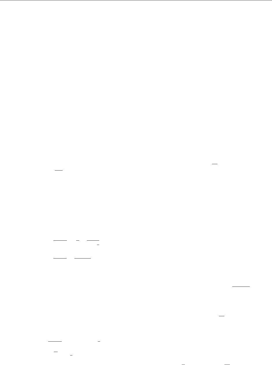
process is illustrated in Figure 2.

A Heegaard diagr am of S

 K determines a

presentation of 

 K) with one generator x

for each -circle and one relator w

for each -circle.

To find the relator w

, one travels along 

recording each intersection with some 

by append-

ing x

1

to the relator. The sign is determined by the

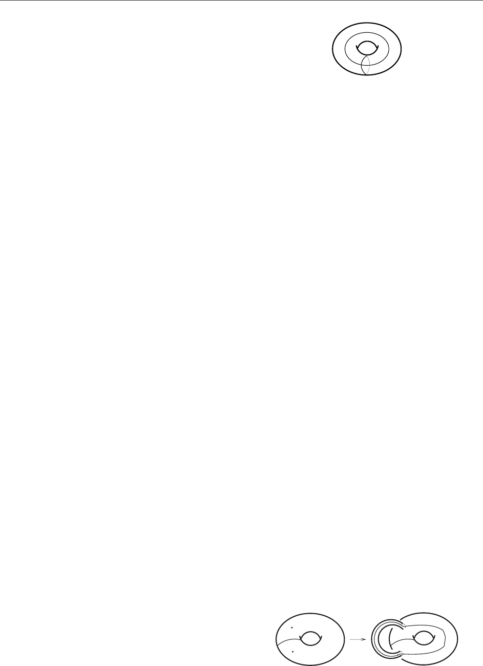
sign of the intersection. As an example, consider the

two doubly pointed diagrams of Figure 3, both of

which correspond to the same Heegaard diagram of

. (It is isotopic to the one shown in Figure 1.) The

fundamental groups of the associated knot comple-

ments can be read off from the corresponding genus-

2 Heegaard splittings. Starting from the point where

Figure 1 Heegaard splitting of S

corresponding to the

standard decomposition of S

into two solid tori.

Figure 2 Going from a doubly pointed diagram to a Heegaard

diagram of the knot complement.

Knot Homologies 211



intersects the left-hand side of the square and

moving to the right, we get



ðS

 K

Þ¼hx

; x

1

¼ 1i



ðS

 K

Þ¼hx

; x

1

¼ 1i

The first group is isomorphic to Z, and the knot in

Figure 3a is the unknot. The second is isomorphic to



of the complement of the trefoil knot, and in fact

the knot in Figure 3b is the left-handed trefoil.

The definition of C

(D) is based on a classi cal

method for computing the Alexander polynomial

known as the Fox calculus, which takes as its input

a presentation of 

 K). According to Fox

calculus,

ðKÞ¼q

detðd

1i;jg

½13

Here d

is an element of the group ring

Z½H

ðS

 KÞ ﬃ Z½q

2



It is determined by the following rules:

¼ 

½14

ab ¼ d

a þjajd

b ½15

1

¼x

1



½16

where

jj: 

ðS

 KÞ!H

ðS

 KÞﬃZ ¼hq

i½17

is the abelianization map. The factor of q

is chosen

so that P

(K)(1) = 1andP

(K)(q) = P

(K)(q

1

As an exampl e, consider the two presentations

above. In the first presentation, jjsends x

to 1 and

to q

,so

1



¼ 1  x

1



þ x

1



¼ 1  1 þ 1

¼ 1 ½18

which is the Alexander polynomial of the unknot. If

we abelianize the relator in the second presentation,

we see that jx

j= jx

j= q

,so

1



¼ x

 x

1



þ x

1



½19

¼ q

 1 þ q

2

½20

which is the Alexander polynomial of the trefoil.

When g = 1, the complex C

(D) is generated by

the points of 

\ 

. These intersection points may

be naturally ident ified with the appearances of the

generator x

in w

, and thus with the monomials

appearing in d

. For example, the three mono-

mials which appear on the right-hand sides of eqns

[18] and [19] correspond, respectively, to the points

labeled p

, p

, and p

in Figure 3. The j-grading of

each generator is given by the exponent of q which

the corresponding monomial contributes to the

Alexander polynomial. Thus, all three generators in

Figure 3a have j-grading 0, while in Figure 3b, the

generators p

, p

,andp

have j-gradings 2, 0, and 2

respectively.

For general g, the monomials appearing in the

determinant of eqn [13] correspond to intersection

points of the two totally real tori  = 



and  = 



inside the symmetric product

Sym

. The knot Floer h omology is the Lagran-

gian Floer homology of  and  inside the

symplectic manifold Sym

(  z  w). The gen era-

tors of C

(D) are the points of  \ ;the

differential is defined by counting holomorphic

disks with boundary on  and . To be precise, for

x 2  \ ,

x ¼

2

ðx;yÞ;ðÞ¼1

ðÞ¼n

ðÞ¼0

#MðÞy ½21

Here 

(x, y) denotes the set of homotopy classes of

maps of the strip D = {a þ ib jb 2 [0, 1]} into Sym



which take the right-hand boundary to  and the

left-hand boundary to , and which limit to x as

b !1 and to y as b !1. () denotes the formal

dimension of the space of pseudoholomorphic disks

in this homotopy class. There is a natural action by

translation on the space of such maps, so when

() = 1 we can divide out by this action and obtain

an oriented zero-dimensional moduli space M().

Finally, by n

() and n

() we denote the intersec-

tion number of such a strip with the divisors

determined by z and w inside of Sym

. The

requirement that they vanish forces the strip to lie

(a) (b)

Figure 3 Doubly pointed Heegaard diagrams for the unknot

and the trefoil. Opposite sides of the square are identified to form

a torus. The dotted line represents 

212 Knot Homologies

in Sym

(  z  w). It can be shown that, for

 2 

(x, y),

jðxÞjðyÞ¼n

ðÞn

ðÞ½22

so j(d

x) = j(x).

When g = 1, computing the differential amounts

to counting maps of the strip into the Heegaard

torus. This can be done algorithmically using the

Riemann mapping theorem, so computation of H

purely combinatorial. Knots of this form are called

(1,1) knots. They are one of our few windows into

the behavior of H

for large knots.

As an example, consider the diagram of Figure 3a.

The two shaded regions represent the domains

of classes 

2 

, p

) and 

2 

, p

The Riemann mapping theorem implies that up

to reparametrization, there is a unique holo-

morphic map of the strip into each region, so

#M(

) = 1 =#M(

). The di fferential in

)isgivenby

ðp

Þ¼p

¼ d

ðp

Þ¼0

and H

(U) ﬃ Z. This reflects the fact that we could

have chosen the more efficient diagram of S

 U

shown in Figure 1, simply by moving 

to remove

two of the intersection points.

For comparison, consider the diagram for the

trefoil shown in Figure 3b. All three generators of

) have different j-gradings, so we must have

 0. Thus, H

(T) ﬃ Z

. The two disks 

and 

are still present, but now n

(

) = n

(

) = 1, so

neither disk contributes to the differential. This is

reflected in the fact that 

cannot be moved to

reduce the number of intersection points without

passing through either z or w.

Deformations

In this case, finding an appropriate deformation of

(D) is simple: we just drop the condition that

() = 0 in the definition of the differential. If a

homotopy class  2 

(x, y) contributes nontrivially

to the sum, it must have a holomorphic representative,

which necessarily intersects the divisor in Sym



defined by z non-negatively. Thus, n

()  0. From

[22], it follows that j(x)  j(y) = n

()  0, so this

new differential has the form d

þ d

, where d

strictly lowers the j-grading.

The fact that the homology of C

(D) with respect

to the perturbed differential is Z goes back to the

knot Floer homology’s roots in Heegaard Floer

homology. By dropping the condition that

() = 0, we have effectively forgotten about the

basepoint z, and thus about the knot. The new

complex simply computes the Heegaard Floer group

HF(S

), which is isomorphic to Z. When g = 1, this

can be seen directly: if we remove the basepoint z,

any genus-1 Heegaard diagram of S

can be isotoped

into the standard diagram of Figure 1.

Construction of H

In this case, the geometric data D needed to define

the chain complex C

(D) is a planar diagram of

the knot, and the classical model on which the

construction of C

(D) is based is the Kauffman state

model for the Jones polynomial. There is a related

homology theory

(D), known as the unreduced

Khovanov homology, whose graded Euler character-

istic is (q þ q

1

(K). This is the original categor-

ification of the Jones polynomial defined in

Khovanov (2000).

To construct

(D), we consider complete resolu-

tions of the planar diagram D. As shown in Figure 4,

there are two different ways to resolve each crossing

of D.IfD has n crossings, there will be 2

ways to

resolve all n, one for each vertex of the cube [0, 1]

To a vertex v, we associate the crossingless planar

diagram D

obtained from the corresponding reso-

lution of D. Thus, each vertex of the cube is

decorated by a 1-manifold D

If e is an edge joining vertices v

and v

(where v

has one more 0 coordinate than v

), we write

e : v

, and decorat e e with a two-dimensional

cobordism S

from D

to D

. S

is a product

cobordism outside a neighborhood of a single

crossing, where it is the one-handle cobordism

between the 0-resolution and the 1-resolution. The

resulting cobordism is necessarily composed of

a union of product cobordisms (cylinders) together

with a single nontrivial cobordism (a pair of pants).

Thus, starting from D, we have constructed an

n-dimensional cube whose vertices are decorated by

1-manifolds and whose edges are decorated by

cobordisms between them . This is the cube of

resolutions of D.

The next step in the construction of

(D)isto

apply a graded (1 þ 1)-dimensional TQFT A to the

cube of resolutions. A is a functor which associates

to each 1-manifold X a group A(X), and to each

two-dimensional cobordism W : X

a homo-

morphism A(W):A(X

) !A(X

). If we apply A to

all the manifolds and cobordisms of the cube of

Figure 4 0- and 1-resolutions of a crossing.

Knot Homologies 213

resolutions, we obtain a new cube, decorated with

groups and cobordisms between them. This process

is summarized in Table 1.

We can now describe the chain complex

(D).

As a group,

ðDÞ¼

AðD

Þ½23

where the sum runs over all vertices of the cube of

resolutions. For x 2A(D

), the differential is given by

x ¼

e:v!v

ð1Þ

sðeÞ

AðS

ÞðxÞ½24

The signs in this sum are determined by assigning a

sign (1)

s(e)

to each edge e in such a way that every

two-dimensional face of the cube has an odd

number of  signs on its edges. (This ensures that

= 0.) There are many ways to do this, but they all

result in isomorphic complexes.

The homological grading i on

(D) is easily

determined. For x 2A(D

), we set i(x) = i(v)  c(D),

where i(v) is the sum of all the coordinates of v, and

c(D) is a constant. Clearly, i(d

x) = i(x) þ 1. In order

to have invariance, it turns out that c(D) must be

chosen to be equal to the number of negative

crossings in D.

It remains to specify the TQFT A. At the level of

groups, A(S

) is a free abelian group of rank 2:

AðS

Þ¼A ¼h1; Xi½25

General principles then imply that





¼ A

n

½26

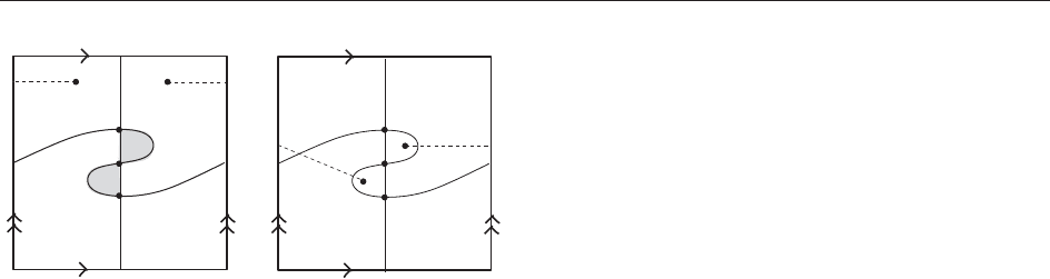
To specify the maps induced by cobordisms, it is

enough to descr ibe the maps associated to the two

pairs of pants shown in Figure 5. They are given by

mð1  1Þ¼1

ð1Þ¼1  X þ X  1 ½27

mð1  XÞ¼mðX  1Þ¼X

ðXÞ¼X  X ½28

mðX  XÞ¼0 ½29

Note that the multiplication m makes A into a

commutative ring isomorphic to Z [X]=(X

A is a graded TQFT. In other words, there is a

grading q on A and its tensor products, determined by

qð1Þ¼1

qða  bÞ¼qðaÞþqðbÞ

½30

qðXÞ¼1 ½31

From eqns [27]–[29], it is easy to see that

qðmða  bÞÞ ¼ qða  bÞ1

qððaÞÞ ¼ qðaÞ1

½32

If we define j(x) = k(D) þ q(x) þ i(x), it follows that

j(d

x) = j(x). Taking the graded Euler characteristic

gives

ð

ðDÞÞ ¼ q

kðDÞ

ðqÞ

iðvÞ

ðq þ q

1

½33

where n

is the number of components of D

.Ifwe

define k(D) to be the writhe of D, this is preci sely

Kauffman’s formula for the unnormalized Jones

polynomial.

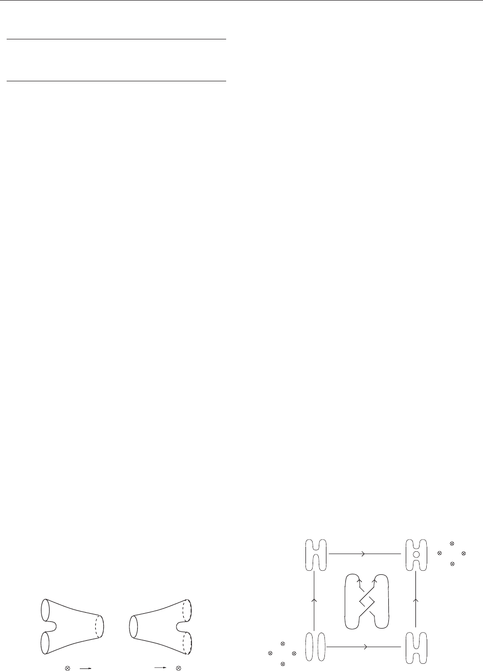
Figure 6 illustrates

(D) for a simple two-

crossing link. The figure shows the original link (in

the center), the cube of resolutions, and basis vectors

for

(D), together with their j-gradings. We leave it

to the reader to check that the homology

(L)is

four dimensional, supported in j-gradings 1 and 3 at

the vertex labeled 00, and in gradings 5 and 7 at the

vertex labeled 11.

Table 1 Summary of cube of resolutions

Vertex v

1- manifold D

Group A(D

)

Edge

Cobordism

Homomorphism

e : v

: D

A(S

) : A(D

) !A(D

)

Am : A A

Δ : A

A A

Figure 5 Maps induced by pairs of pants.

01 11

= 1

= 3

= 5

= 3

= 5

= 7

= 5

= 3

= 5

= 3

Figure 6 The cube of resolutions for the Hopf link.

214 Knot Homologies

To get the reduced chain complex C

(D), we must

divide the graded Euler characteristic by a factor of

(q þ q

1

). This is accomplished by choosing a

marked point on K and requiring that for each

resolution D

, the vector associated to the circle

containing the marked point lie in the subspace of A

spanned by X.IfD is a diagram of a knot, the

resulting homology H

(K) is independent of the

choice of marked poin t. For links, H

(L) depends on

the component of the link on which the marked

point lies.

Deformations

Deformations in the N = 2 theory are constructed

using a technique introduced by E S Lee. The idea is

to replace the graded TQF T A wi th a filtered TQFT

. As a group, we still have A(S

) = A, but the

multiplication and comultiplication maps are per-

turbations of those for A:

ð1 1Þ¼1



ð1Þ¼1 X þX 1 r1 1 ½34

ð1  XÞ¼m

ðX  1Þ¼X



ðXÞ¼X  X þs1  1 ½35

ðX  XÞ¼rX þ s ½36

The new terms involving r and s have q gradings

strictly greater than the terms which are shared with

eqns [27]–[29]. Thus, the differential defined by

replacing m and  by m

and 

will be a

perturbation of the original differential on

(D).

The simplicity of the homol ogy with respect to the

new differential depends on the fact that when the

polynomial X

 rX  s has simple roots, the TQFT

decomposes as a direct sum of two one-

dimensional TQFTs. This implies that for a knot,

the deformed homology

(K) decomposes as a

direct sum of two copies of H

(K). This group is

always isomorphic to Z,so

(K) ﬃ Z  Z.Ifs = 0,

the same strategy can be used to define deformations

of the reduced chain complex C

(D). In this case, we

find that the deformed homology is isomorphic to a

single copy of Z.

See also: Floer Homology; Gauge Theory: Mathematical

Applications; The Jones Polynomial; Knot Theory and

Physics; Topological Quantum Field Theory: Overview.