Francoise J.-P., Naber G.L., Tsun T.S. (editors) Encyclopedia of Mathematical Physics

Подождите немного. Документ загружается.

which acts on the Siegel space H

M ¼



:  7!ðA þ BÞðC þ DÞ

1

Here A, ..., D are g  g blocks .

The rows of the matrix  define a rank-2g lattice



in C

and the Jacobian of C is the torus

JðCÞ¼C



More intrinsically, one can define J(C) as follow s.

Let H

(C, !

) be the space of holom orphic differ-

ential forms on C. Then, integration over cycles

defines a monomorphism

ðC; ZÞ!H

ðC;!



 7!



and

JðC Þ¼H

ðC;!



ðC; ZÞ

For a fixed base point P

2 C, the Abel–Jacobi

map is defined by

u : C ! JðCÞ

P 7!

; ...;



Here, the integration is taken over some path

from P

to P. Obviously, the integral dep ends on

the choice of this path, but since J(C)was

obtained by dividing ou t the periods given by

integrating over a basis of H

(C, Z), the map is

well defined.

Let C

be the dth Cartesian product of C, that is,

the set of all ordered d-tuples (P

, ..., P

). Then, u

defines a map

: C

! JðCÞ

ðP

; ...; P

Þ7!uðP

ÞþþuðP

where þ is the usual addition on the torus J(C).

If d = g 1, then

 ¼ Imðu

g1

ÞJðCÞ

is a hypersurface (i.e., has codimension 1 in J(C))

and is called a theta divisor. A different choice of the

base point P

results in a trans lation of the theta

divisor. Using the theta divisor, one can show that

J(C) is an abelian variety, that is, J(C) can be

embedded into some projective space P

. The pair

(J(C), ) is a principally polarized abelian variety

and Torelli’s theorem states that C can be

reconstructed from its Jacobian J(C) and the theta

divisor .

Divisors, Linear Systems,

and Line Bundles

A divisor D on C is a formal sum

D ¼ n

þþn

; P

2 C; n

2 Z

The degree of D is defined as

deg D ¼ n

þþn

and D is called ‘‘effective’’ if all n

 0. Every

meromorphic function f 6¼ 0 defines a divisor

ðf Þ¼f

 f

where f

are the zeros of f and f

the poles (each

counted with multiplicity). Divisors of the form (f )are

called principal divisors and the degree of any principal

divisor is 0 (see the next section). Two divisors D

and

are called linearly equivalent (D

 D

)iftheir

difference is a principal divisor, that is,

 D

¼ðf Þ

for some meromorphic function f 6¼ 0. This defines

an equivalence relation on the group Div(C) of all

divisors on C. Since principal divisors have degree 0,

the notion of degree also makes sense for classes of

linearly equivalent divisors. We define the divisor

class group of C by

ClðCÞ¼DivðCÞ=

The degree map defines an exact sequence

0 ! Cl

ðCÞ!ClðCÞ

deg

Z ! 0

where Cl

classes of degree 0.

Let C

be the set of unordered d-tuples of points

on C, that is,

¼ C

where the symmetric group S

acts on the Cartesian

product C

by permutation. This is again a smooth

projective variety and the Abel–Jacobi map

: C

! J(C) clearly factors through a map

: C

! JðCÞ

The fibers of this map are of particular interest.

Theorem 2 (Abel). Two effective divisors D

and

on C of the same degree d are linearly equivalent

if and only if u

) = u

One normally denotes the inverse image of u

(D)by

jDj¼u

1

ðu

ðDÞÞ ¼ D

; D

 0; D

 D

Note that the latter description also makes sense if

D itself is not necessarily effective. One calls jDj the

422 Riemann Surfaces

complete linear system defined by the divisor D.If

deg D < 0, then automatically jDj= ;, but the

converse is not necessarily true. Let M

be the

field of meromorphic (or equivalently rational)

functions on C. Then, one defines

LðDÞ¼ f 2M

; ðf ÞD

This is a C-vector space and it is not difficult to see

that L(D) has finite dimension. To every function

0 6¼ f 2 L(D), one can associate the effective divisor

¼ðf ÞþD  0

Clearly, D

 D and every effective divisor with this

property arises in this way. This gives a bijection

PðLðDÞÞ ¼ jDj

showing that the complete linear system jDj has the

structure of a projective space. A linear system is a

projective subspace of some complete linear system jDj.

Clearly, the map u

: C

! J(C) can be extended

to the set Div

theorem then states that this map factors through

(C), that is, that we have a commutative diagram

Div

(C )Cl

(C )

J(C

)

where u

is injective.

Theorem 3 (Jacobi’s Inversion Theorem). The

map u

is surjective and hence induces an isomorphism

: Cl

ðCÞﬃJðCÞ

It should be noted that the definition of the maps

depends on the choice of a base point P

2 C.

Hence, the maps

are not canonical, with the

exception of the isomorphism

:Cl

where the choice of P

drops out.

The concepts of divisors and linear systems can be

rephrased in the language of line bundles. A (holo-

morphic) vector bundle on a complex manifold M is a

complex manifold E together with a projection

p : E ! M which is a locally trivial C

-bundle. This

means that an open covering (U



)

2A

of M and local

trivializations

–1

)

≅ p

exist, such that the transition maps

’



 ’

1



ðU





ÞC

ðU



\ U



ÞC

!ðU



\ U



ÞC

are fiberwise linear isomorphisms. If M is connected,

then r is constant and is called the rank of the vector

bundle. A line bundle is simply a rank-1 vector bundle.

Alternatively, one can view vector bundles as

locally free O

-modules, where O

denotes the

structure sheaf of holomorphic (or in the algebro-

geometric setting regular) functions on M.An

-module E is called locally free of rank r,ifan

open covering (U



)

2A

of M exists such that Ej



ﬃ

r



. The transition functions of a locally free sheaf

can be used to define a vector bundle and vice versa,

and hence the concepts of vector bundles and locally

free sheaves can be used interchangeably. The open

coverings U



can be viewed either in the complex

topology, or, if M is an algebraic variety, in

the Zariski topology, thus leading to either holo-

morphic vector bundles (locally free sheaves in the

C-topology) or algebraic vector bundles (locally free

sheaves in the Zariski topology). Clearly, every

algebraic vector bundle defines a holomorph ic

vector bundle. Conversely, on a projective variety

M, Serre’s GAGA theorem (ge´ome´trie alge´briques et

ge´ome´trie analytique), a vast generalization of

Chow’s theorem, states that there exists a bijection

between the equivalence classes of algebraic and

holomorphic vector bundles (locally free sheaves).

The Picard group Pic M is the set of all isomorph-

ism classes of line bundles on M. The tensor product

defines a group structure on Pic M where the neutral

element is the trivial line bundle O

and the inverse

of a line bundle L is its dual bundle L



, which is also

denoted by L

1

. For this reason, locally free sheaves

of rank 1 are also called invertible sheaves.

We now return to the case of a compact Riemann

surface (algebraic curve) C. The concept of line

bundles and divisors can be trans lated into each

other. If D =

is a divisor on C and U an open

set, then we denote by D

the restriction of D to U,

that is, the divisor consisting of all points P

2 U

with multiplicity n

. One then defines a locally free

sheaf (line bundle) L(D)by

LðDÞðUÞ¼ f 2M

ðUÞ; ðf ÞD

To see that this is locally free, it is enough to

consider for each point P

a neighborhood U

which a holomorphic function t

exists, which

vanishes only at P

and there of order 1 (i.e., it is a

local parameter near the point P

). Then,

LðDÞðU

Þ¼t

n

ﬃO

This correspondence defines a map

Div C ! Pic C

D 7!LðDÞ

Riemann Surfaces 423

It is not hard to show that:

1. every line bundle L2Pic C is of the form L=

L(D) for some divisor D on the curve C;

2. D

 D

() L (D

) ﬃL(D

);

3. L(D

) L(D

) ﬃL(D

þ D

); and

4. L(D) ﬃL(D)

1

Hence, there is an isomorphism of abelian groups

ClðCÞﬃPic C

This correspondence allows to define the degree of a

line bundle L. In the complex analytic setting this

can also be interpreted as follows. Let O



be the

sheaf of nowhere-vanishing functions. Using cocycles,

one easily identifies

ðC; O



ÞﬃPic C

and the exponential sequence

0 ! Z !O

exp



! 0

induces an exact sequence

0 ! H

ðC; ZÞ!H

ðC; O

! H

ðC; O



Þ¼Pic C ! H

ðC; ZÞ

The last map in this exact sequence associates to

each line bundle L its first Chern class c

(L) 2

(C, Z) ﬃ Z, which can be identified with the

degree of L. Hence, the subgroup Pic

C of degree 0

line bundles on C is isomorphic to

Pic

C ﬃ H

ðC; O

Þ=H

ðC; ZÞ

Altogether there are identifications

Pic

C ﬃ Cl

C ﬃ JðCÞ

The Riemann–Roch Theorem

and Applications

For every divisor D on a compact Riemann surface C,

the discussion of the preceding section shows that there

is an identification of finite-dimensional vector spaces

LðDÞ¼H

ðC; LðD ÞÞ

where H

(C, L(D)) is the space of global sections of

the line bundle L(D). One defines

lðDÞ¼dim

LðDÞ

It is a crucial question in the theory of compact Riemann

surfaces to study the dimension l(D)asD varies.

The canonical bundle !

of C is defined as the dual

of the tangent bundle of C. Its global sections are

holomorphic 1-forms. Every divisor K

on C with

= L(K

) is called (a) canonical divisor. The

canonical divisors are the divisors of the meromorphic

1-forms on C, whereas the effective canonical divisors

correspond to the divisors of holomorphic 1-forms

(here, we simply write a 1-form locally as f (z)dz and

define a divisor by taking the zeros, resp. poles of f (z)).

By abuse of notation, we also denote the divisor class

corresponding to canonical divisors by K

. There is a

natural identification

PðH

ðC;!

ÞÞ ¼ jK

For a divisor D, the index of speciality is defined by

iðDÞ¼l ðK

 DÞ¼dim

LðK

 DÞ

The linear system jK

 Dj is called the adjoint

system of jDj. A crucial role is played by the

Theorem 4 (Riemann–Roch). For any divisor D on a

compact Riemann surface C of genus g, the equality

lðDÞi ðDÞ¼deg D þ 1  g ½2

holds.

This can also be written in terms of line bundles.

If L is any line bundle, then we denote the

dimension of the space of global sect ions by

ðLÞ ¼ dim

ðC; LÞ

Then, the Riemann–Roch theorem can be written as

ðLÞ  h

ð!

L

1

Þ¼deg Lþ1  g ½3

This can be written yet again in a different way, if

we use sheaf cohomology. By Serre dua lity, there is

an isomorphism of cohomology groups

ðC; LÞ ﬃ H

ðC;!

L

1



and hence if we set

ðLÞ¼ dim

ðC; LÞ

then [3] reads

ðLÞ  h

ðLÞ ¼ deg Lþ1  g ½4

Whereas [2] is the classical formulation of the

Riemann–Roch theorem, formula [4] is the formula-

tion which is more suitable for genera lizations.

From this point of view, the classical Riemann–

Roch theorem is a combination of the cohomologi-

cal formulation [4] together with Serre duality.

The Riemann–Roch theorem has been vastly gen-

eralized. This was first achieved by Hirzebruch who

proved what is nowadays called the Hirzebruch–

Riemann–Roch theorem for vector bundles on projec-

tive manifolds. A further generalization is due to

Grothendieck, who proved a ‘‘relative’’ version invol-

ving maps between varieties. Nowadays, theorems like

the Hirzebruch–Riemann–Roch theorem can be

424 Riemann Surfaces

viewed as special cases of the Atiyah–Singer index

theorem for elliptic operators. The latter also contains

the Gauss–Bonnet theorem from differential geometry

as a special case. Moreover, Serre duality holds in

much greater generality, namely for coherent sheaves

on projective varieties.

Applying the Riemann–Roc h theorem [3] to the

zero divisor D = 0, resp. the trivial line bundle O

one obtains

ð!

Þ¼g ½5

that is, the number of independent global holo-

morphic 1-forms equals the genus of the curve C.

Similarly, for D = K

, resp. L= !

, we find from [3]

and [5] that

deg K

¼ 2g  2

These relations show, how the Riemann–Roch

theorem links analytic, resp. algebraic, invariants

with the topology of the curve C.

Finally, if deg D > 2g  2, then deg(K

 D) < 0

and hence i(D) = l(K

 D) = 0and[2] becomes

lðDÞ¼deg D þ 1  g if deg D > 2g  2

which is Riemann’s original version of the theorem.

Classically, linear series arose in the study of

projective embeddings of algebraic curves. For a

nonzero effective divisor

D ¼

i¼1

; n

> 0

the support of D is defined by

suppðDÞ¼ P

; ...; P

A complete linear system jDj is called base point

free, if no point P exists which is in the support of

every divisor D

2jDj. This is the same as saying

that for every P 2 C a section s 2 H

(C, L(D)) exists

which does not vanish at P. Let jDj be base point

free and let s

, ..., s

2 H

(C, L(D)) be a basis of the

space of sections. Then, one obtains a map

’

jDj

: C ! PðH

ðC; LðD ÞÞÞ ¼ P

P 7!ðs

ðPÞ : ... : s

ðPÞÞ

The divisors D

2jDj are then exactly the pullbacks

of the hyperplanes H of P

under the map ’

jDj

. Note

that the map ’

jDj

as defined here depends on the

choice of the basis s

, ..., s

, but any two such

choices only differ by an automorphism of P

.We

say that jDj, resp. the associated line bundle

L= L(D), is very ample if ’

jDj

defines an

embedding. Using the Riemann– Roch theorem, it is

not difficult to prove:

Proposition 1 Let D be a divisor of degree d on the

curve C. Then

(i) jDj is base point free if d  2g and

(ii) jDj is very ample if d  2g þ 1.

If the genus g(C)  2, then one can prove that jK

is base point free and consider the canonical map

’

: C ! P

g1

A curve C is called hyperelliptic if there exists a

surjective map f : C ! P

which is a covering of

degree 2. In genus 2 every curve is hyperelliptic,

whereas for genus g  3 hyperelliptic curves are

special. The connection with the canonical map is

given by

Theorem 5 (Clifford). Let C be a curve of genus

g  2. Then the canonical map is an embedding if

and only if C is not hyperelliptic.

We end this section by stating Hurwitz’s theorem:

Let f : C ! D be a surjective holomorphic map

between compact Riemann surfaces (if f is not

constant then it is automatically surjective). Then,

near a point P 2 C the map f is given in local

analytic coordinates by f (t) = t

and we call f

‘‘ramified’’ of order n

if n

> 1. The ramificat ion

divisor of f is defined as

R ¼

P2C

ðn

 1ÞP

Note that this is a finite sum. If we define



ðQÞ¼

P2f

1

ðQÞ

then one can show that

deg f ¼ deg f



ðQÞ¼

P2f

1

ðQÞ

is independent of the point Q. This number is called

the degree of the map f. (This should not be

confused with the degree deg(f ) of the principal

divisor (f ) defined by f.) In fact, applying the above

equality to the map f : C ! P

associated to a

nonconstant meromorphic function f shows that

the degree of the principal divisor (f ) is zero, since

degðf Þ¼deg f



ð0Þdeg f



ð1Þ ¼ 0

Theorem 6 (Hurwitz). Let f : C ! D be a surjec-

tive holomorphic map between compact Riemann

surfaces of genus g(C) and g(D), respectively. Then,

2gðCÞ2 ¼ deg f ð2gðDÞ2 Þþdeg R

where R is the ramification divisor .

Riemann Surfaces 425

Brill–Noether Theory

In this section, we state the main results of Brill–

Noether theory. For a divisor D on a curve C we

denote by

rðDÞ¼lðDÞ1

the projective dimension of the complete linear

system jDj. The principal objects of Brill–Noether

theory are the sets W

 Cl

ðCÞ¼ D; deg D ¼ d; rðDÞr

These sets are subvarieties of Cl

(C).

We denote by g

a linear system (not necessarily

complete) of degree d and projective dimension r.

Closely related to the varieties W

are the sets

ðCÞ¼ ;  is a g

on C



These sets also have a natural structure as a projective

variety. Clearly, there are maps G

(C).

If g = g(C) is the genus of the curve C, then the

Brill–Noether number is defined as

ðg; r; dÞ¼g ðr þ 1Þðg  d þ rÞ

Its significance is that it is the expected dimension of

the varieties G

(C). The two basic results of Brill–

Noether theory are:

Theorem 7 (Existence Theorem). Let C be a curve

of genus g. Let d, r be integers such that d  1, r  0,

and (g, r, d)  0. Then G

nonempty and every component of G

sion at least . If r  d  g, thenthesameistrue

for W

(C).

Theorem 8 (Connectedness Theorem). Let C be

a curve of genus g and d, r integers such that d  1,

r  0, and (g, r, d)  1. Then G

The above theorems hold for all curves C. There

are other theorems which only hold for general

curves (where general means outside a countable

union of proper subvarieties in the moduli space, see

the section ‘‘Modul i of compact Riem ann surfa ces’’).

Theorem 9 (Dimension Theorem). Let C be a

general curve of genus g and d  1, r  0 integers. If

(g, r, d ) < 0, then G

component of G

Theorem 10 (Smoothness Theorem). Let C be a

general curve of genus g and d  1, r  0. Then,

Brill–Noether theory started with a paper of Brill

and Noether in 1873. It was, however, only from

the 1970s onwards that the main theorems could be

proved rigorously, due to the work of Griffiths,

Harris, Kleiman, Mumford, and many others. For

an extensive treatment of the theory, as well as a list

of references, the reader is referre d to Arbarello

et al. (1985).

Green’s Conjecture

In recent years, much progress was a chieved i n

understanding the equations of canonical c urves. If

the curve C is not hyperelliptic, then the canonical

map ’

: C ! P

g1

defines an embedding. We

shall, in this case, identify C with its image in P

g1

and call this a canonical curve. The Clifford index

(for a precise definition see Lazarsfeld (1989))isa

first measure of how special a curve C is with

respect to the canonical map. Hyperelliptic curves,

where t he canonical map fails to be an embedding,

have, by definition, Clifford index 0. The two next

special cases are plane quintic curves (they have

a g

) and trigonal c urves. A curve C is called

trigonal, if there is a 3 : 1 map C ! P

,inwhich

case C has a g

. More generally, the gonality of a

curve C is the minimal degree of a surjective map

C ! P

. Plane quintics and trigonal curves are

precisely the curves w hich have Clifford index 1.

Theorem 11 (Enriques–Babbage). If C  P

g1

is a

canonical curve, then C is either defined by quad-

ratic equations, or it is trigonal or isomorphic to a

plane quintic curve (i.e., it has Clifford index 1).

One can now ask more refined questions about

the equations defining canonical curves and the

relations (syzygies) among these equations. This

leads to looking at the minimal free resolution of a

canonical curve C, which is of the form

0 I



g1 ðjÞ



 

g1 ðjÞ



Here, I

is the ideal sheaf of C and O

g1

(n)isthe

nth power of the dual of the Hopf bundle (or

tautological sub-bundle) on P

g1

if n  0,

resp. the jnjth power of the Hopf bundle if n <

0. The 

The Green conjecture predicts a link between the

nonvanishing of certain Betti numbers and geo-

metric properties of the canonical curve, such as

the existence of multisecants. Rec ently, C Voisin

and M Teixidor have proved the Green conjecture

for general curves of given gonality (see Beauville

(2003)).

426 Riemann Surfaces

Moduli of Compact Riemann Surfaces

As a set, the moduli space of compact Riemann

surfaces of genus g is defined as

¼ C; C is a compact

Riemann surface of genus gg=ﬃ

For genus g = 0, the only Riemann surface is the

Riemann sphere

C = P

and hence M

consists of

one point only. Every Riemann surface of genus 1 is

a torus

E ¼ C=L

for some lattice L, which can be written in the form



¼ Z þ Z; Im >0

Two elliptic curves E



= C=L



and E



= C=L



are

isomorphic if and only if a matrix

M ¼



2 SLð2; ZÞ

exists with



a þ b

c þ d

This proves that

¼ H

=SLð2; ZÞ

and this construction also shows that M

can itself

be given the structure of a Riemann surface. Using

the j-function, one obtains that

ﬃ C

The situation is considerably more complicated for

genus g  2. The space of infinitesimal deformations

of a curve C is given by H

(C, T

) where T

is the

tangent bundle. By Serre duality

ðC; T

ÞﬃH

ðC;!

2



and by Riemann’s theorem it then follows that

dim H

ðC; T

Þ¼dim H

ðC;!

2

Þ¼3g  3

This shows that a curve of genus g depends on

3g  3 parameters or moduli, a dimension count

which was first performed by Riemann.

In genus 2 every curve has the hyperelliptic

involution, and for a genera l curve of genus 2 this

is the only automorphism. In genus g  3 the

general curve has no automorphisms, but some

curves do. The order of the automorphism group is

bounded by 84(g  1). The existence of automorph-

ism for some curves means that M

is not a

manifold, but has singularities. The singularities

are, however, fairly mild. Locally, M

always

looks like C

3g3

=G near the origin, where G is a

finite group acting linearly on C

3g3

. One expresses

this by saying that M

has only finite quot ient

singularities. A space with this property is also

sometimes referred to as a V-manifold or an

orbifold. Moreover, M

is a quasiprojective variety,

that is, a Zariski-open subset of a projective variety.

As the above parameter count implies, the dimen-

sion of M

is 3g  3. At this point it can also be

clarified what is meant by a general curve in the

context of Brill– Noether theory: a property is said to

hold for the general curve in Brill–Noether theory if

it holds outside a countable number of proper

subvarieties of M

It is often useful to work with projective, rather

than quasiprojective, varieties. This means that one

wants to compactify M

to a projective variety M

preferably in such a way that the points one adds

still correspond to geometric objects. The crucial

concept in this context is that of a stable curve. A

stable curve of genus g is a one-dimensional

projective variety with the follo wing properties:

1. C is connected (but not necessarily irreducible),

2. C has at most nodal singularities (i.e., two local

analytic branches meet transversally),

3. the arithmetic genus p

(C, O

) = g, and

4. the automorphism group Aut(C)ofC is finite.

The last of these cond itions is equivalent to the

following: if a component of C is an elliptic curve,

then this must either meet another component or

have a node, and if a component is a rational curve,

then this component must either have at least two

nodes or one node and intersect another component,

or it is smooth and has at least three points of

intersection with other components.

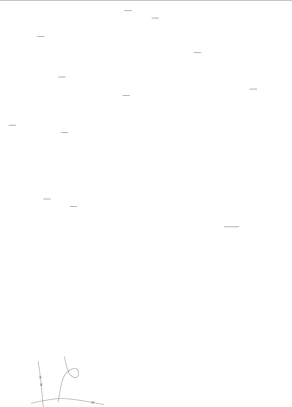
It should be noted that, in contrast to the previous

illustrations, Figure 5 is drawn from the complex

point of view, that is, the curves appear as one-

dimensional objects.

The concept of stable curves leads to what is

generally known as the Deli gne–Mumford compac -

tification of M

¼fC; C is a stable curve of genus gg=ﬃ

g = 0

= 2

Figure 5 An example of a stable curve of genus 3.

Riemann Surfaces 427

Theorem 12 (Deligne–Mumford, Knudsen). M

an irreducible, projective variety of dimension 3g  3

with only finite quotient singularities.

The spaces

have been studied intensively over

the last 30 years. From the point of view of

classification, an important question is to determine

the Kodaira dimension of these spaces.

Theorem 13 (Harris–Mumford, Eisenbud–Harris).

The moduli spaces

are of general type for

g > 23.

On the other hand, it is known that

rational for g  6, unirational for g  14, and has

negative Kodaira dimension for g  16.

A further topic is to understand the cohomology

, resp. the Chow ring, and to compute the

intersection theory on

. For these topics we refer

the reader to Vakil (2003).

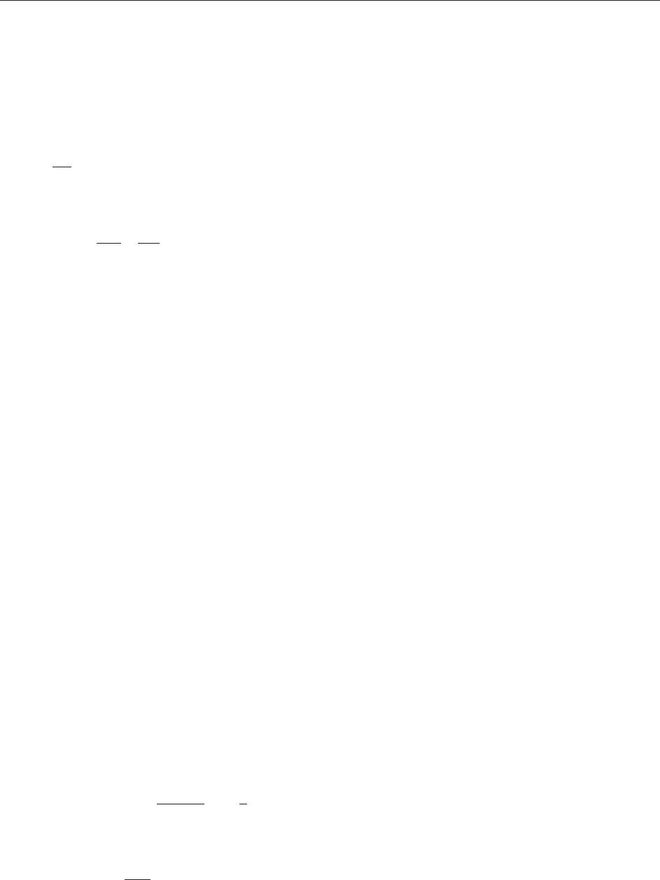
Closely related is the moduli problem of stable

n-pointed curves. A stable n-pointed curve (Figure 6)

is an (n þ 1)-tuple (C, x

, ..., x

), where C is a

connected nodal curve and x

, ..., x

are smooth

points of C with the stability condition that the

automorphism group of ( C, x

, ..., x

) is finite.

These curves can be parametrized by a coarse

moduli space

g, n

. These spaces share many

properties of the spaces

: they are irreducible,

projective varieties with finite quotient singularities

and of dimension 3g  3 þ n.

A further development, which has become very

importantinrecentyears,isthatofmodulispacesof

stable maps. These were introduced by Kontsevich in

the context of quantum cohomology. To define stable

maps, one first fixes a projective variety X and then

considers (n þ 2)-tuples (C, x

, ..., x

, f ) where

(C, x

, ..., x

)isann-pointed curve of genus g and

f : C ! X a map. The stability condition is, that this

object allows only finitely many automorphisms

’ : C ! C, fixing the marked points x

, ..., x

,such

that f  ’ = f . In order to obtain meaningful moduli

spaces, one also fixes a class  2 H

(X, Z). One then

asks for a space parametrizing all stable (n þ 2)-tuples

(C, x

, ..., x

, f ) with the additional property that



[C] = . This construction is best treated in the

language of stacks, and one can show that this moduli

problem gives rise to a proper Deligne–Mumford stack

g, n

(X, ). In general, this stack is very complicated,

it need not be connected, can be very singular, and may

have several components of different dimensions. Its

expected dimension is

exp : dim

g; n

ðX;Þ

¼ðdim X  3Þð1  gÞþn þ



ðT

Quantum cohomology can now be rephrased as

intersection theory on the stack

g, n

(X, ). In

general, these stacks do not have the expected

dimension. For this reason, Behrend and Fantechi

(1997) have constructed a virtual fundamental class of

the right dimension, which is the correct tool for the

intersection theory which gives the algebro-geometric

definition of quantum cohomology. In addition to this,

there is also a symplectic formulation. It was shown by

B Siebert that both approaches coincide.

Verlinde Formula and Conformal Blocks

The study of vector bundles (locally free sheaves) on

a compact Riemann surface is an area of research in

its own right. For a rank-r bundle E, the slope of E is

defined by

ðEÞ ¼

deg E

where the degree of E is defined as the degree of the

line bundle

E = det E. The bundle E is called

stable, resp. semistable, if

ðFÞ <ðEÞ; resp:ðFÞ  ðEÞ

for every proper sub-bundle {0} $ F $ E.LetC be a

compact Riemann surface of genus g  2 and let

(r) be the moduli space of semistable rank-r vector

bundles with trivial determinant det E = O

.Thisis

a projective variety of dimension (r

 1)(g  1).

It contains a smooth open set, whose points corres-

pond to the isomorphism classes of stable vector

bundles. The complement of this set is in general the

singular locus of SU

(r) and its points correspond to

direct sums of line bundles of degree 0. These are the

so-calledgradedobjectsofthesemistable,butnot

stable, bundles. By a theorem of Narasimhan and

Seshadri, the points of SU

(r) are also in one-to-one

correspondence with the isomorphism classes of

representations 

Let L 2 Pic

g1

g  1onC. Then, the set



¼E2SU

ðrÞ; dim H

ðC; ELÞ > 0



g = 2

= 0

Figure 6 An example of marked stable curve.

428 Riemann Surfaces

is a Cartier divisor on SU

(r) and thus defines a line

bundle L on SU

(r). This is a natural generalization

of the construction of the classical theta divisor. The

line bundle L generates the Picard group of the

moduli space SU

(r).

Theorem 14 (Verlinde Formula). If C has genus g

and k is a positive integer, then

dim H

ðSU

ðrÞ; L

r þ k



StT¼f1;...;rþkg

jSj¼r

s2S

t2T



sin 

s  t

r þ k



g1

This formula was first found by Verlinde in the context

of conformal field theory. Due to this relationship, the

spaces H

(SU

(r), L

) are also called conformal

blocks. These spaces can also be defined for principal

bundles. Rigorous proofs for the general case of the

Verlinde formula are due to Beauville–Laszlo and

Faltings. For a survey, see Beauville (1995).

See also: Characteristic Classes; Cohomology Theories;

Index Theorems; Mirror Symmetry: a Geometric Survey;

Moduli Spaces: An Introduction; Polygonal Billiards;

Several Complex Variables: Basic Geometric Theory;

Several Complex Variables: Compact Manifolds;

Topological Gravity, Two-Dimensional.

Further Reading

Arbarello E, Cornalba M, Griffiths Ph, and Harris J (1985)

Geometry of Algebraic Curves, vol. I. New York: Springer.

Beauville A (1995) Vector bundles on curves and generalized

theta functions: recent results and open problems. In: Boutet

de Montel A and Morchenko V (eds.) Current Topics in

Complex Algebraic Geometry, (Berkeley, CA, 1992/93),

Math. Sci. Res. Inst. Publ., vol. 28, pp. 17–33. Cambridge:

Cambridge University Press.

Beauville A (2003) La conjecture de green ge´ne´rique [d’apre`s

C. Voisin]. Expose´ 924 du Se´minaire Bourbaki.

Behrend K and Fantechi B (1997) The intrinsic normal cone.

Inventiones Mathematicae 128: 45–88.

Faber C and Looijenga E (1999) Remarks on moduli of curves. In:

Faber C and Looijenga E (eds.) Moduli of Curves and Abelian

Varieties, Aspects Math. E33, pp. 23–45. Braunschweig: Vieweg.

Farkas H and Kra I (1992) Riemann Surfaces, 2nd edn. New

York: Springer.

Forster O (1991) Lectures on Riemann Surfaces (translated from

the 1977 German Original by Bruce Gilligan), Reprint of the

1981 English Translation. New York: Springer.

Griffiths Ph and Harris J (1994) Principles of Algebraic

Geometry, Reprint of the 1978 Edition, Wiley Classics

Library. New York: Wiley.

Hartshorne R (1977) Algebraic Geometry. Heidelberg: Springer.

Jost J (1997) Compact Riemann Surfaces. An Introduction to

Contemporary Mathematics (translated from the German

Manuscript by Simha RR). Berlin: Springer.

Kirwan F (1992) Complex Algebraic Curves. Cambridge:

Cambridge University Press.

Lazarsfeld R (1989) A sampling of vector bundle techniques in the

study of linear series. In: Cornalba M, Gomez-Mont X, and

Verjovsk (eds.) Lectures on Riemann Surfaces, pp. 500–559.

Teaneck, NJ: World Scientific.

Miranda R (1995) Algebraic Curves and Riemann Surfaces.

Providence: American Mathematical Society.

Mumford D (1995) Algebraic Geometry. I. Complex Projective

Varieties, Reprint of the 1976 Edition. Berlin: Springer.

Vakil R (2003) The moduli space of curves and its tautological

ring. Notices of the American Mathematical Society 50(6):

647–658.

Weyl H (1997) Die Idee der Riemannschen Fla¨ che (Reprint of the

1913 German Original, With Essays by Reinhold Remmert,

Michael Schneider, Stefan Hildebrandt, Klaus Hulek and

Samuel Patterson. Edited and with a Preface and a Biography

of Weyl by Remmert). Stuttgart: Teubner.

Riemann–Hilbert Methods in Integrable Systems

D Shepelsky, Institute for Low Temperature Physics

and Engineering, Kharkov, Ukraine

Introduction

The Riemann–Hilbert (RH) method in mathematical

physics and analysis consists in reducing a particular

problem to the problem of reconstruction of an

analytic, scalar- or matrix-val ued function in the

complex plane from a prescribed jump across a

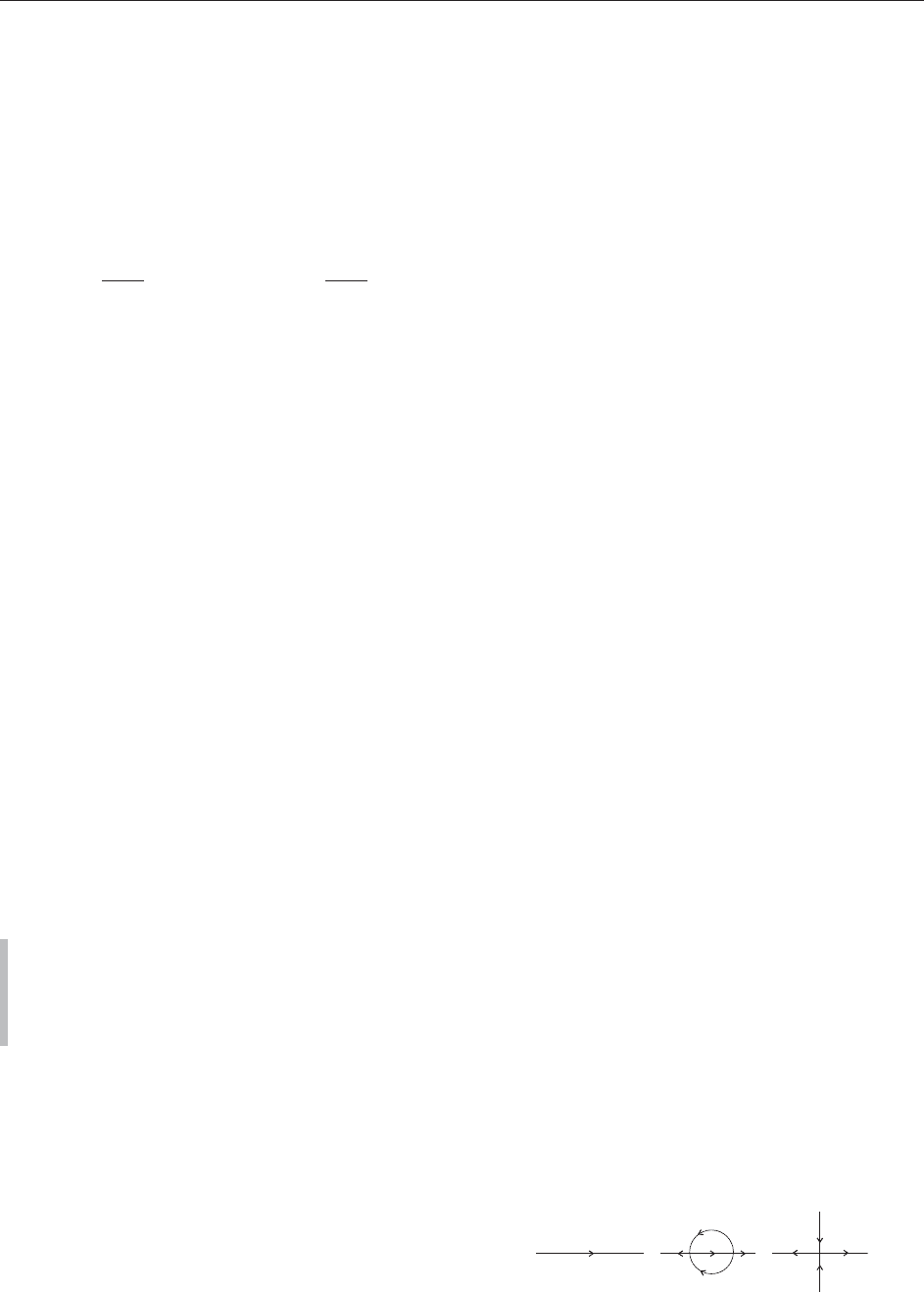
given curve. More precisely, let an oriented contour

 be given in the complex -plane. The contour 

may have points of self-intersections, and it may

consist of several connected components; typical

contours appearing in applications to integrable

systems are shown in Figure 1.

The orientation of an arc in  defines the þ

and the  side of . Suppose in addition that we

are g iven a map v :  !GL(N, C)withv, v

1

(). The ( normalized) RH problem determined

by the pair (, v) consists in finding an N  N

Figure 1 Typical contours for RH problems.

Riemann–Hilbert Methods in Integrable Systems 429

matrix-valued function m() with the following

properties:

mðÞ is analytic in Cn ½1a

ðÞ¼m



ðÞvðÞ for  2 

where m

ðÞðm



ðÞÞ is the limit

of m from the þ ðÞ side of  ½1b

mðÞ!I (identity matrix) as  !1 ½1c

The precise sense in which the limit at 1 and the

boundary values m



are attained are technical

matter that should be specified for each given RH

problem (, v).

Concerning the name RH problem we note that

in literature (particularly, in the theory of bound-

ary values of analytic functions), the problem of

reconstructing a f unction from its jump across a

curve is often called th e Hilbert bou ndary-value

problem. The closely related problem of analytic

matrix factorization (given  and v,findG()

analytic and nondegenerate in Cn such that



= v on ) is sometimes called the Riemann

problem. The name ‘‘RH problem’’ is also

attributed to the reconstruction of a Fuchsian

system with given poles and a given monodromy

group.

In applications, the jump matrix v also depends

on certain parameters, in which the original problem

at hand is naturally formulated (e.g., v = v(; x, t)in

applications to the integrable nonlinear differential

equations in dim ension 1 þ 1, with x being the space

variable an d t the time variable), and the main

concern is the behavior of the solution of the RH

problem, m(; x, t), as a function of x and t.

Particular interest is in the behavior of m(; x, t)as

x and t become large.

In the scalar case, N = 1, rewriting the original

multiplicative jump condition in the additive form

log m

ðÞ¼log m

ðÞþlog vðÞ

and using the Cauchy–Plemelj–Sokhotskii formula

give an explicit integral representation for the

solution

mðÞ¼exp

2i



log vð Þ

  

d



½2

(in the case of nonzero index,  log vj



6¼ 0, formula

[2] admits a suitable modification).

A generic (nonabelian) matrix RH problem

cannot be solved explicitly in terms of contour

integrals; however, it can always be reduced to a

system of linear singular-integral equations, thus

linearizing an originally nonlinear system.

The main benefit of reducing an originally non-

linear problem to the analytic factorization of a

given mat rix function arises in asymptotic analysis.

Typically, the dependence of the jump matrix on the

external parameters (say, x and t) is oscillatory. In

analogy of asymptotic evaluation of oscillatory

contour integrals via the classical method of steepest

descent, in the asymptotic evaluation of the solution

m(; x, t) of the matrix RH problem as x, t !1, the

nonlinear steepest-descent method examines the

analytic structure of the jump matrix v(; x, t)in

order to deform the contour  to contours where

the oscillatory factors become exponentially small as

x, t !1, and hence the original RH problem

reduces to a collection of local RH problems

associated with the relevant points of stationary

phase. Although the method has (in the matrix case)

noncommutative and nonlinear elements, the final

result of the analysis is as efficient as the asymptotic

evaluation of the oscillatory inte grals.

Dressing Method

The RH method allows describing the solution of a

differential system independently of the theory of

differential equations. The solution might be expli-

cit, that is, given in terms of elementary or elliptic or

abelian functions and contour integrals of such

functions. In general (transce ndental) case, the

solution can be represented in terms of the solution

of certain linear singular integral equations.

In the modern theory of integrable systems, a

system of nonlinear differential equations is often

called integrable if it can be represented as a

compatibility condition of an auxiliary overdeter-

mined linear system of differential equations called a

Lax pair of the given nonlinear system (actually it

might involve more than two linear equations). In

order that the compatibility condition represents a

nontrivial nonlinear system of equations, the Lax

pair is required to depend rationally on an auxiliary

parameter (called a spectral parameter). The RH

problem formulated in the complex plane of the

spectral parameter allows, given a particular solu-

tion of the compatibility equa tions, to construct

directly new solutions of the compatibility system by

‘‘dressing’’ the initial one.

For example, let D(x, ), x 2 R

,  2 C be an N  N

diagonal, polynomial in  with smooth coefficients,

function such that a

:= @D=@x

are polynomials in

 of degree d

. Then 

:= exp D(x, ) solves the

system of linear equations @

=@x

= a



, whose

compatibility conditions @



=@x

= @



=@x

are trivially satisfied. Given a contour  and a smooth

function v, consider the matrix RH problem [1]

430 Riemann–Hilbert Methods in Integrable Systems

with the jump matrix

v(; x):= expD(x, )v ()

exp D(x, ). Let m(; x ) be the solution of this RH

problem. Then (D

= (D



v,whereD

f :=

@f =@x

þ [a

, f ]with[a, b]:= ab  ba. The Liouville

theorem implies that (D

m)m

1

is an entire function

which is o(

)as !1.Setting(x, ):= m(; x)

exp D(x, ) gives the system of linear equations

@

¼ a

k<d



ðxÞR

ðx;Þ ½3

the compatibility conditions for which are



¼½R

; R

½4

Equating coefficients of variou s powers of  in [4]

gives a (generally) nonlinear system of partial

differential equations for the coefficient matrices

. Thus, given D(x, ), the RH problem, if it is

solvable, maps the pair (, v) to solutions of [4].

Specializing to n = 2 with variab les (x, t) 2 R

, the

overdetermined system of linear equations and the

corresponding compatibility conditions are



¼ U; 

¼ V ½5

and

 V

þ½U; V¼0 ½6

respectively. Conditions [6] are sometimes called the

zero-curvature conditions.

Equations [5] and [6] with U and V depending

rationally on the spectral parameter  represents the

integrable nonlinear systems in 1 þ 1 dimension. A

typical example of such a system is the (defocusing)

nonlinear Schro¨ dinger (NLS) equation

þ q

 2jqj

q ¼ 0 ½7

Starting from the RH problem with the 2  2 jump

matrix

vð; x; tÞ¼e

i

vðÞe

i

½8

where (; x, t) = t

þ x, 

= diag{1, 1}, and

v() satisfies the involution 



()

= v(



),

expanding out the limit of the solution of the RH

problem as  !1

mð; x; tÞ¼I þ

ðx; tÞ



þ o





½9

and arguing as above gives [5], with

U ¼

i

0 q



q 0

½10

and q = i(m

)

, whereas the compatibility condi-

tion [6] reduces to [7].

The relation between the RH problem and the

differential equations [5] is local in x and t; it is based

only on the unique solvability of the RH problem,

the Liouville theorem, and the explicit dependence of

the jump matrix in x and t. The uniqueness of the

solution of an RH problem is basically provided by

the Liouville theorem: the ratio m

(1)

(2)

)

1

of any

two solutions is analytic in Cn and continuous

across  and is therefore identically equal to I by the

normalization condition [1c].

On the other hand, there are no completely

general effective criteria for the solvability. Never-

theless, many RH problems seen in applications to

integrable syst ems satisfy the following sufficient

condition: if  is symmetric with respect to R and

contains R, and if, in addition, v



() = v(



) for  2

nR and Re v()>0 for  2 R, then the RH

problem is solvable.

For nonlinear equations supporting solitons, the

RH problem appears naturally in a more general

setting, as a meromorphi c factorization problem,

where m in [1] is sought to be a (piecewise)

meromorphic function, with additionally prescribed

poles and respective residue conditions. Alterna-

tively, in the Riemann factorization problem



= v, one assumes that G degenerates at

some given points 

, ..., 

2 

and 

, ..., 





, where C =

[ 



[ , and prescribes two sets

of subspaces, Im Gj

 = 

and Ker Gj

 = 

. In the case

v  I, the solution of the factorization problem with

zeros (meromorphic RH problem) is purely alge-

braic, and gives formulas describing multisoliton

solutions. In the general case, v 6 I, the mero-

morphic RH problem can be algebraically converted

to a holomorphic RH problem, by subsequently

removing the poles with the help of the Blaschke–

Potapov factors.

Alternatively, a meromorphic RH problem can be

converted to a holomorphic one by adding to  an

additional contour 

aux

enclosing all the poles,

interpolating the constan ts involved in the residue

conditions inside the region surrounded by 

aux

, and

defining a new jump matrix on 

aux

using the

interpolant and the Blaschke–Potapov factors.

RH problems formulated on the complex plane C

correspond typically to solutions of relevant non-

linear problems decaying at infinity. For other types

of boundary conditions (e.g., nonzero constants or

periodic or quasiperiodic boundary conditions), the

corresponding RH problem is naturally formulated

on a Riemann surface. For example, the RH

problem associated with finite density conditions

q(x, t) !e

i



as x !1 for the NLS equation [7]

is naturally formulated on the two-sheet Riemann

surface of the function k() =

ﬃﬃﬃﬃﬃﬃﬃﬃﬃﬃﬃﬃﬃﬃﬃﬃﬃﬃ



 4

with

Riemann–Hilbert Methods in Integrable Systems 431