Graef M. Introduction to conventional transmission electron microscopy
Подождите немного. Документ загружается.


148 The transmission electron microscope
equations and they are rather difficult to solve because of the explicit dependence
of the relativistic mass on the velocity components. The non-relativistic version of
these equations is obtained by setting m = m
0
.
The second equation can be rewritten by noting that [Rei93]
1
r
d(mr
2
˙ϕ)
dt
=
d(mr ˙ϕ)
dt
+ m
˙
r ˙ϕ.
This can be verified easily by explicitly writing out the two derivatives. If we
truncate the expressions for the field components B
r
and B
z
(equations 3.5 and 3.6)
after the first term, then we find for equation (3.12):
1
r
d(mr
2
˙ϕ)
dt
=
|e|
2
$
r
˙
B(z) − 2
˙
rB(z)
%
,
which reduces to
d(mr
2
˙ϕ)
dt
=
|e|
2
d
$
r
2
B(z)
%
dt
.
This can be integrated readily to give
r
2
m ˙ϕ −
|e|
2
B(z)
= C, (3.14)
where C is an integration constant.
†
C must be zero for any trajectory that intersects
the optical axis at some point (for such a point r = 0). Such trajectories are known
as meridional trajectories. Trajectories that are not meridional are skew trajectories.
C can be computed for an arbitrary initial point with coordinates (r
0
,ϕ
0
, z
0
).
3.4.4 The paraxial approximation
It is common practice to transform the time dependence of the equations of motion
into a dependence on one of the coordinates. In most cases the z-coordinate is taken
to be the independent variable, and the goal of the calculation is then to determine
r(z) and ϕ(z) for a charged particle traveling through the field described by B(z).
The azimuthal equation can be rewritten using the following relation:
d
dt
=
˙
z
d
dz
= v
d
dz
,
where v is the axial velocity of the electron. It is a good approximation to as-
sume that v is very nearly constant, so that
¨
z = ˙v = 0. In what follows we will
†
If we had chosen to derive the equations of motion from the variational principle, then this equation would have
followed directly from the fact that the coordinate variable ϕ does not explicitly appear in the Lagrangian of the
system, and therefore ˙ϕ must be a constant of motion [Szi88].
3.4 Basic electron optics: round magnetic lenses 149
denote a derivative with respect to z by a prime, i.e. d f /dz ≡ f
. The azimuthal
equation (3.14) for a meridional trajectory (C = 0) becomes
˙ϕ −
|e|
2mv
B(z) = ˙ϕ −
|e|
2
2em
0
ˆ
B(z) = 0.
Using the notation of the previous chapter we find
˙ϕ −
ηB(z)
2
√
ˆ
= 0.
(3.15)
The total rotation angle of the electron trajectory around the optical axis is derived
by integrating this equation:
ϕ(z) = ϕ
0
+
η
2
√
ˆ
.
z
z
0
B(z)dz. (3.16)
The rotational frequency for a paraxial electron intersecting the optical axis can
then be derived from equation (3.14),
˙ϕ =
e
2m
B(z),
and this quantity is known as the Larmor frequency.
The radial equation can be simplified using the so-called paraxial approxima-
tion: we will only consider electrons traveling close to the optical axis (r remains
small), with motion predominantly in the z-direction (both radial and azimuthal
velocities are small compared to the forward velocity, or r
1; r ϕ
1). The
radial trajectory equation (3.11) can then be rewritten using the following relation:
¨
r = v
2
r
+r
¨
z ≈ v
2
r
.
Since ˙v = 0, we also have
˙
m = 0, and we leave it as an exercise for the reader to
show that this leads to the following radial paraxial equation:
r
+
η
2
B
2
(z)
4
ˆ
r = 0.
(3.17)
It is important to note that the prefactor
η
2
B
2
(z)
4
ˆ
in the radial paraxial equation is always positive, and becomes equal to zero only
for a vanishing magnetic field strength. This implies that an electron trajectory is
150 The transmission electron microscope
always bent towards the optical axis (for a round lens),
†
regardless of the electron
energy and the details of the magnetic field configuration.
3.4.5 Numerical trajectory computation
The radial equation (3.17) can be solved analytically for a few particular choices
of the axial magnetic flux distribution B(z), but in general requires a numerical
approach. We refer to [HK89a, HK89b] for a detailed discussion of the analytical
solutions for Glaser’s bell-shaped field, given by
B(z) =
B
0
1 +
(
z/a
)
2
.
B
0
2a
a is a parameter with the dimension of length, which indicates the extent of the field:
small values of a correspond to sharply peaked fields. Although this field does not
represent a realistic magnetic field distribution (the field strength does not drop off
sufficiently fast at large distances), it is often employed in theoretical calculations
because it allows closed-form solutions for almost all relevant parameters, including
the lens aberrations.
In this section we opt for a simple numerical approach to determine the paraxial
electron trajectory for an arbitrary axial field distribution B(z). From the
website
the reader may download the program lens.f90, which implements a simple paraxial
meridional trajectory computation. The program is written for Glaser’s bell-shaped
field, but can be modified easily for other axial field distributions. The reader is
encouraged to modify the field parameters to study how a magnetic field can be
used to create lenses with varying focal length. It is particularly interesting to
use
lens.f90 to simulate how a two-condensor lens system works. The following
paragraphs describe the program and the PostScript output.
The program
lens.f90 integrates both the azimuthal and radial equations. The
azimuthal equation is straightforward to solve by replacing the integral (3.16) by a
summation. There are many different algorithms which can be used in this case:
trapezoidal integration, Simpson’s rule, Romberg integration and Gaussian quadra-
ture are amongst the more commonly used methods [Szi88]. Since we will be
using fourth-order Runge–Kutta method to solve the radial equation, we will use
Simpson’s rule for the azimuthal equation.
‡
If the integration interval (z
0
, z
N
)is
†
A positive second term in the radial equation can only be canceled by a negative first term, which means that
the curvature of the trajectory must be negative, i.e. the electron trajectory bends towards the optical axis.
‡
It can be shown that Simpson’s rule is equivalent to a fourth-order Runge–Kutta method.

3.4 Basic electron optics: round magnetic lenses 151
divided into N segments of length z, then the total rotation angle ϕ(z
N
)isgiven
by [AS77]
ϕ(z
N
) = ϕ
0
+
ηz
6
√
ˆ
+
B(z
0
) + B
(
z
N
)
+ 2
N/2−1
j=1
B
(
z
0
+ 2 jz
)
+ 4
N/2
j=1
B
(
z
0
+
(
2 j − 1
)
z
)
,
+ O
$
(
z
)
4
%
(3.18)
with ϕ
0
the initial rotation angle at the point z
0
. The error in the computation
is of order (z)
4
, as indicated by the last term. This equation is rather simple
to implement in a Fortran routine. In the same computational loop, we can also
calculate an approximate value for the focal length, using Busch’s formula [Bus26]:
1
f
=
η
2
4
ˆ
.
z
N
z
0
B
2
(z)dz; (3.19)
=
η
2
z
12
ˆ
+
B
2
(z
0
) + B
2
(z
N
) + 2
N/2−1
j=1
B
2
(z
0
+ 2 jz)
+4
N/2
j=1
B
2
(z
0
+ (2 j − 1)z)
,
+ O
$
(
z
)
4
%
.
Both numerical values can then be compared
†
with the theoretical values for Glaser’s
bell-shaped field [HK89a]:
ϕ =
ηB
0
2
√
ˆ
πa;
1
f
=
η
2
B
2
0
8
ˆ
πa.
The program
lens.f90 employs fourth-order Runge–Kutta integration with fixed
step size to integrate the radial paraxial equation (the public domain
rksuite90
software package is available from the www.netlib.org website; for a gen-
eral description of Runge–Kutta procedures we refer the interested reader to the
Numerical Recipes book [PFTV89]). The Runge–Kutta procedure operates on a
†
In comparing these equations with others quoted in the literature for Glaser’s bell-shaped field one should bear
in mind that there is a difference between the real focal length and the asymptotic focal length. The equations
above all refer to asymptotic quantities. Since Glaser’s field has a slow drop off at large distances from the
maximum field strength, the numerical procedure will in general underestimate the total rotation angle ϕ and
overestimate the focal length.

152 The transmission electron microscope
system of two coupled first-order differential equations which are equivalent to the
radial equations:
dy
1
dz
= y
2
; (3.20)
dy
2
dz
=−
η
2
B
2
(z)
4
ˆ
y
1
, (3.21)
from which the solution r(z) = y
1
follows. The function y
1
provides the distance
from the optical axis, and the function y
2
represents the slope of the electron
trajectory with respect to the optical axis. The initial values to be inserted into
this routine are then the initial distance r(z
0
) and slope r
(z
0
).
Pseudo Code PC-11 Simulation of paraxial meridional electron trajectories.
Input: axial flux density B(z), acceleration voltage
Output: PostScript drawing of trajectories
integrate rotation angle ϕ(z) and focal length f {equation 3.18}
use a fourth-order Runge–Kutta procedure {equations 3.20 and 3.21}
(
rksuite.f) to obtain r(z)
generate PostScript output
The source code of the lens.f90 program is rather simple and is represented in
pseudo code
PC-11 ; the radial equation is solved by a driver subroutine rksol2. The
initial values are taken to be r(z
0
) = 1.0 and r
(z
0
) = 0.0, i.e. an electron entering
the field parallel to the optical axis at unit distance. The initial value for the azimuthal
angle is taken as ϕ(z
0
) = π/2, i.e. the electron enters the field traveling in the plane
(y, z).
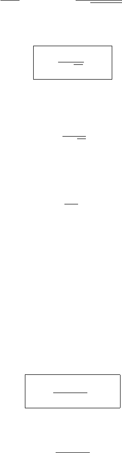
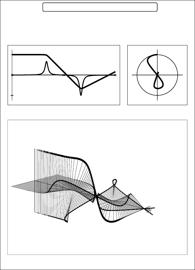
The output of the program is a PostScript file (default name:
lens.ps) which can
be displayed with a PostScript viewer or sent directly to a printer. Typical program
output is shown in Fig. 3.5. The list near the top of the page shows the acceleration
voltage (both the input value and the relativistic value), the electron wavelength, the
maximum axial field strength along the trajectory, the total azimuthal rotation angle
ϕ(z
N
), and the focal length computed using Busch’s formula. The three rectangular
boxes show:
(i) top left: profile of the axial field distribution B(z) (arbitrary scale, thinnest line), and
the radial trajectory r(z) (thickest line). When the radial distance becomes larger than
a preset truncation value, the trajectory is clipped;
(ii) top right: projection of the trajectory along the positive z-direction (i.e. looking away
from the electron source). The position of each point is given by (x(z), y(z)) =
(r(z) cos ϕ(z), r(z) sin ϕ(z));
3.4 Basic electron optics: round magnetic lenses 153
z
x
y
Electron Trajectory Computation
Written by MDG, 1998.
Voltage [V] 100000.0000
Relativistic voltage [V] 109784.7500
Wavelength [pm] 3.7014
Total rotation [rad] 2.4584
Focal length [mm] 0.7973
B(z), r(z)
Radial plot
B-max [T] 2.0000
5.0 mm
x
y
Azimuthal plot
Perspective plot
5.0 mm
0
-
Fig. 3.5. Representative output of the lens.f program, for Glaser’s bell-shaped field. The
parameters of the field are B
max
= 2.0T,a = 1.0 mm, and the acceleration voltage is
V = 100 kV.
(iii) bottom: perspective representation of four identical trajectories, obtained from the
computed trajectory by rotation by [0, 1, 2, 3] × π/2 in the (x, y) plane. The trajecto-
ries are clipped by the frame of the drawing, to prevent them from overlapping other
parts of the output.
154 The transmission electron microscope
B(z), r(z)
Radial plot
x
y
Azimuthal plot
B(z), r(z)
x
y
B(z), r(z)
-5.0 mm
x
y
100
100
200
200
400
400
5.0 mm
0
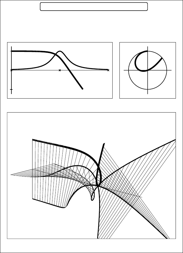
Fig. 3.6. Radial and azimuthal trajectories for the field of Fig. 3.5, for acceleration voltages
V = 100, 200 and 400 kV.
This program can be used to study how various parameters affect the focal length of
the lens and the electron trajectory. For instance, by entering a number of different
acceleration voltages for a given lens field, we find (Fig. 3.6) that a faster electron is
less affected by the field or, equivalently, that a higher acceleration voltage requires
more powerful lenses, or lenses that act over a longer distance along the electron
trajectory.
Stationary (i.e. time-independent) magnetic fields cannot accelerate electrons,
they can only change the travel direction of the electrons. Accordingly, in the
absence of electrostatic fields, magnetic fields leave the energy of the electron
unchanged. The action of an axially symmetric magnetic field on the trajectory
of an electron can then be understood as follows: for an electron with an initial
axial velocity component v
z
, the radial component of the magnetic flux density
B
r
creates an azimuthal force F
ϕ
. The particle thus acquires an azimuthal velocity
component v
ϕ
= r ˙ϕ, which will make the trajectory curve around the optical axis.
This azimuthal component will then interact with the z component of the flux
density to create a radial force component F
r
, which brings the particle closer to
the optical axis.
If we place two lenses along the optical axis the electron trajectory becomes
more complex. Figure 3.7 shows a configuration of two lenses (B
1,max
= 1.2T,
B
2,max
=−1.8T,a = 1.0 mm), spaced by 20 mm. The acceleration voltage is
V = 400 kV. This configuration mimics a double-condensor system, where the
first lens has a fixed cross-over and the second a variable cross-over; by changing
the current through the second lens the focal length of the system can be changed.
Note that the negative magnitude of the second field does not affect the focal length,
but does change the overall rotation angle.
The programs discussed in this section are greatly simplified versions of the
types of computations a lens designer would have to carry out to create an entire
3.4 Basic electron optics: round magnetic lenses 155
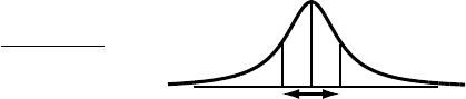
Electron Trajectory Computation
Written by MDG, 1998.
Voltage [V] 400000.0000
Relativistic voltage [V] 556556.0625
Wavelength [pm] 1.6439
Total rotation [rad] −0.3657
B(z), r(z)
Radial plot
B-max [T] 1.7970
-30 mm
x
y
Azimuthal plot
Perspective plot
z
x
y
30 mm
0
Fig. 3.7. Double-lens configuration; the centers of the lenses are 20 mm apart. The pa-
rameters of the field are B
max
= 1.2, −1.8T,a = 1.0 mm, and the acceleration voltage is
V = 400 kV.
microscope column, or any other lens configuration. Professional designers would
typically employ variable step-size Runge–Kutta integration algorithms or the
Burlisch–Stoer algorithm [PFTV89] to integrate the equations of motion accu-
rately for realistic field distributions. Although most microscopists will rarely need
156 The transmission electron microscope
to worry about the physics of a magnetic lens, it is useful to play with simple
programs such as
lens.f90 to acquire some understanding of how a magnetic lens
works.
3.4.6 General properties of round magnetic lenses
The general solution to any second-order differential equation (and therefore also
equation 3.17) can be written as a linear combination of two independent solutions.
We select two solutions with special properties:
†
the first solution, r
1
(z), satisfies
the condition
lim
z→−∞
r
1
(z) = 1, (3.22)
or, the incident ray is asymptotically parallel to the optical axis, at unit distance
from the axis. The second solution, r
2
(z), is asymptotically parallel to the outgoing
optical axis, i.e.
lim
z→+∞
r
2
(z) = 1. (3.23)
A general solution of equation (3.17) thus has the form:
r(z) = Ar
1
(z) + Br
2
(z). (3.24)
We will refer to each solution as a ray. Since magnetic fields have infinite range, a
ray can only become asymptotically identical to a straight line.
The rays r
1
(z) and r
2
(z) become asymptotically straight lines far from the lens
center, and hence we have (using the equation for a straight line intersecting the
optical axis):
lim
z→+∞
r
1
(z) = (z − z
Fi
)r
1i
;
lim
z→−∞
r
2
(z) = (z − z
Fo
)r
2o
.
We will call z
Fi
the asymptotic image focus (see Fig. 3.8) and z
Fo
the asymptotic
object focus. As before, a prime denotes differentiation with respect to z.
A ray parallel to r
1
(z), but at a different distance from the optical axis, can be
written as λr
1
(z), where λ is a real number; the asymptotic outgoing ray belonging
to λr
1
(z)isλ(z − z
Fi
)r
1i
, according to the relations above. This ray intersects the
optical axis in the same point z
Fi
, hence the name image focus.
We can now determine the intersection of the incident asymptote to the ray
r
1
(z) and its emergent asymptote; the intersection point lies in the plane z = z
Pi
†
We will follow closely Section 16.2 in [HK89a] and Chapter 4 in [Szi88], but with a slightly different notation.
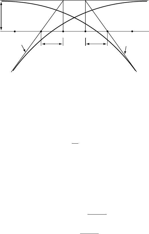
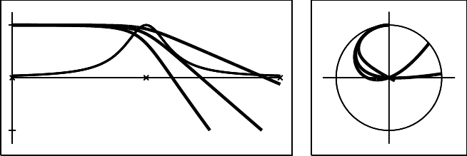
3.4 Basic electron optics: round magnetic lenses 157
r (z) r (z)
1
2
1
slope r'
1i
slope r'
2o
Fo
Pi
Po
Fi
z
z
zz
f
f
o
i
z
z
2
1
Fig. 3.8. Definition of the asymptotic ray parameters and location of the general points z
1
and z
2
.
(see Fig. 3.8), which is called the asymptotic principal image plane:
incident asymptote → 1 = (z
Pi
− z
Fi
)r
1i
← emerging asymptote, (3.25)
from which
z
Pi
= z
Fi
+
1
r
1i
= z
Fi
− f
i
, (3.26)
where f
i
is the asymptotic focal length. Similarly, the asymptotes to r
2
(z) intersect
in the asymptotic principal object plane z = z
Po
, with associated asymptotic focal
length f
o
= 1/r
2o
. The equality f
i
= f
o
is valid, provided the electron does not
experience any change in its kinetic energy while traveling through the lens. Insert-
ing the limit values for r
1
(z) and r
2
(z) into equation (3.24), we obtain the following
equations for the asymptotic general ray:
lim
z→−∞
r(z) = A + B
z − z
Fo
f
o
;
lim
z→+∞
r(z) =−A
z − z
Fi
f
i
+ B.
There are two components to each ray: the distance to the optical axis, and the angle
of the trajectory with respect to the optical axis. It is then convenient to introduce
a two-component ray-vector:
U(z) =
r(z)
r
(z)
. (3.27)
We leave it up to the reader to eliminate A and B from equation (3.27), for two
positions z
1
and z
2
(see Fig. 3.8), z
1
somewhere on the incident asymptote and
z
2
somewhere on the emergent asymptote of the general solution. We obtain the