Graef M. Introduction to conventional transmission electron microscopy
Подождите немного. Документ загружается.


158 The transmission electron microscope
matrix equation
U
2
= T U
1
, (3.28)
where T is the lens transfer matrix, which describes the paraxial behavior of the
lens. The matrix is given explicitly by
T =
−(z
2
−z
Fi
)
f
i
f
o
+
(z
1
−z
Fo
)(z
2
−z
Fi
)
f
i
−
1
f
i
(z
1
−z
Fo
)
f
i
. (3.29)
The transfer matrix can be used as a compact tool to describe the relevant imaging
features of the lens. For a system with multiple lenses sharing the same optical
axis, the image plane of one lens becomes the object plane of the next lens, and we
can describe the behavior of the entire system by multiplication of the individual
transfer matrices in the proper order. The paraxial (asymptotic) imaging properties
of an entire microscope column can thus be reduced to a set of transfer matrices.
Let us now consider a few important special cases. The points z
1
and z
2
used to
determine the transfer matrix T are randomly chosen on the incident and emerging
asymptotes. Consider a point P
o
in the plane z
1
= z
o
, such that all rays leaving P
o
converge to a single point P
i
in the plane z
2
= z
i
. The two planes z
o
and z
i
are
then said to be conjugate planes. Mathematically, this means that the component
r(z
i
) of the ray-vector U
2
(z
i
) must be independent of the initial slope r
(z
o
) of the
trajectory, or, equivalently
(
z
o
− z
Fo
)(
z
i
− z
Fi
)
=−f
i
f
o
. (3.30)
This relation is known as Newton’s lens equation, and it plays a central role in both
light and electron optics [BW75]. In the absence of electrostatic fields (i.e. when
f
o
/ f
i
= 1) the transfer matrix relation for conjugate planes can be rewritten as
r
i
r
i
=
M 0
−1/ f
i
M
α
r
o
r
o
. (3.31)
These equations are interpreted as follows: the radial image distance from the optical
axis is related to the object distance by the relation
r
i
= Mr
o
.
M is hence known as the transverse magnification. It is easy to see that the transverse
magnification depends on the location of the image plane z = z
i
according to
M =−(z
i
− z
Fi
)/ f
i
. In particular, the transverse magnification can be smaller than
1 when the distance between image and principal image planes is shorter than the
focal length. In such a case M is a demagnification factor.

3.4 Basic electron optics: round magnetic lenses 159
The slopes of the trajectories at the object and image locations are related by
r
i
=−
r
o
f
i
+ M
α
r
o
,
where M
α
is the angular magnification. The angular magnification depends on the
location of the object plane z = z
o
according to M
α
= (z
o
− z
Fo
)/ f
i
.
Since the determinant of the transfer matrix is equal to f
o
/ f
i
= 1, we can easily
show (using Newton’s lens equation 3.30) that
MM
α
=
f
o
f
i
= 1.
We thus find that a lens with a large transverse magnification must have a small
angular magnification and vice versa. We will see later on in this chapter that
the objective lens of a TEM is a strongly excited lens with a large transverse
magnification.
In addition to the two focal planes z = z
Fo
and z = z
Fi
, we can define the
following pairs of planes:
r
principal planes: the two conjugate planes related to each other by a unit transverse
magnification are known as the principal planes. They are denoted in Fig. 3.8 by the
symbols z = z
Po
and z = z
Pi
;
r
nodal planes: the nodal planes are located at the intersection points of asymptotic rays for
which the slopes of the incident and emergent sections are equal. The points are related
to each other by unit angular magnification, and are indicated by the symbols z = z
No
and z = z
Ni
. For round magnetic lenses the nodal points coincide with the principal
points [HK89a].
Because of the positive character of the factor η
2
B
2
(z)/4
ˆ
in the radial trajectory
equation, the image nodal point is located closer to the object than the object
nodal point, from which it follows that both nodal and principal planes for a round
magnetic lens are crossed (i.e. the image principal plane is closer to the object plane
than to the image plane).
The various points (focal, principal, and nodal) are collectively called the asymp-
totic cardinal elements of the lens. Using the lens transfer matrix it is straightforward
to compute the magnification properties of a set of coaxial lenses, by direct matrix
multiplication. The theory derived in this section is valid when the details of the
field inside the lens are unimportant, i.e. when one is only interested in the input
and output of a lens. This is the case for most lenses in the TEM, except for the
objective lens.
The objective lens cannot be treated in the same way as the other lenses, since the
specimen is inserted into the magnetic field, thereby dividing the lens into two parts.
For this case, we can use the so-called osculating cardinal elements; this is beyond
160 The transmission electron microscope
Pi
Ni
Po
No
f
i
FiFo
f
o
P
Q
1
2
3
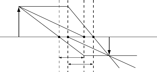
Fig. 3.9. Graphical construction of the image Q of an object point P, using the asymptotic
cardinal elements. Any two of
the three rays shown can be used
to determine the location
Q.
the scope of this textbook and we refer to [Szi88], [Spe88] and [HK89a, Chapter 17]
for more detailed information.
The relations between the cardinal elements and the focal lengths can be used to
determine graphically the image formed by a lens for an arbitrary object location.
Consider the drawing in Fig. 3.9: an object (arrow ending in P) is located to the
left of the lens. The six cardinal elements of the lens are indicated on the drawing
(with crossed principal planes). The image point Q corresponding to P can then be
determined by constructing any two out of the three rays shown in the figure. Ray 1
is drawn parallel to the optical axis until it reaches the image principal plane Pi; then
a straight line is drawn from this intersection point through the image focal point Fi.
Ray 2 is a straight line through the object focal point Fo until it reaches the object
principal plane Po, from where the line is continued parallel to the optical axis into
image space. The third ray 3 goes from the point P to the object nodal point No;a
parallel line is then drawn starting in the image nodal point Ni and continues into
image space. The three lines intersect each other at the image point Q conjugate to
P. For the particular location of P in this drawing, the transverse magnification is
less than one, and the image is a demagnified (and inverted) version of the object.
By varying the current through a magnetic lens, one can change the location of the
focal planes continuously, and therefore the position of the image plane conjugate to
the object. In particular, if the distance between the object and the object focal plane
is less than the object focal length, the image will be magnified rather than demag-
nified. The image space focal plane is commonly known as the back focal plane.
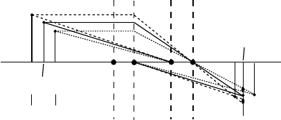
The graphical construction of Fig. 3.9 can be used to illustrate the concepts of
depth of field and depth of focus. Consider three points in an object, shown in
Fig. 3.10. The middle point (o
2
) lies in the object plane conjugate to the image
plane z
2
. The point o
1
to the left is at a larger distance from the lens plane, and
3.4 Basic electron optics: round magnetic lenses 161
o
1
o
2
o
3
D
o
z
1
z
2
z
3
P
i
P
o
F
i
F
o
Fig. 3.10. Graphical illustration of depth of field.
its image plane is therefore to the left of the plane z = z
2
. The point o
3
has its
conjugate image plane at z = z
3
. Since we observe the image in the plane z = z
2
,
the rays originating from the points o
1
and o
3
intersect the image plane z = z
2
in
circles, commonly known as circles of confusion. The radius of a circle of confusion
depends on the range of angles α
o
between the optical axis and the electron rays
that give rise to the image; a smaller angular range produces a smaller circle of
confusion. In optical photography this is typically obtained by reducing the size
of the aperture, i.e. “stopping down” the aperture. It can be shown that the depth
of field D
o
, the distance in object space over which the rays will give rise to an
in-focus image with a circle of confusion smaller than δ, is given by D
o
= 2δ/α
o
,
where α
o
is the semi-aperture angle [WC96,HHN
+
77]. In other words, if we wish to
resolve features of the order of δ = 1 nm, and the largest angle between the electron
trajectories and the optical axis is α
o
= 10 mrad, then the depth of field is given
by D
o
= 200 nm. All the object details larger than δ = 1 nm are simultaneously in
focus if the sample thickness is less than D
o
= 200 nm, when the apertures limit
the maximum angle to 10 mrad. The depth of focus D
i
is the distance in image
space corresponding to D
o
in object space. It is easy to show that D
i
= D
o
M
2
,
where M is the lateral magnification. For a magnification of M = 10
5
, the depth
of focus for the parameters above is D
i
= 2 × 10
12
nm = 2 km, which means that
the precise location of the image plane is not important since the image will be in-
focus over a distance of 2 km! The large depth of focus makes it possible to observe
an in-focus image on the fluorescent screen of the microscope, and then expose
a negative located several centimeters below the image screen without having to
refocus the image. We will return to the circle of confusion concept when we define
the resolution of a microscope in Chapter 10.
3.4.7 Lenses and Fourier transforms
In the preceding sections, we have described how magnetic lenses work, using a
geometrical description. In view of the particle–wave duality of quantum mechanics
we must also consider the action of a lens in terms of the wave function of the
162 The transmission electron microscope
∆
u
(x, y, u)
u
OP
v
x
z
ff
(0, 0, u)
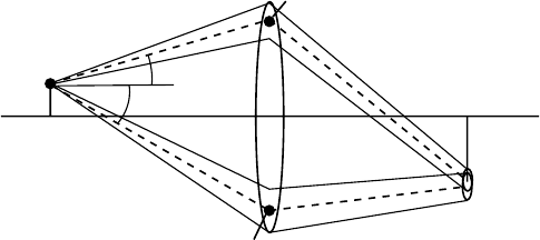
Fig. 3.11. Schematic illustration of the action of a perfect lens. The y-direction comes out
of the plane of the drawing.
electrons passing through the lens. This leads to the field of wave optics. At this
point, we will introduce only briefly the most important concepts of wave optics;
we will return to wave optics in Chapter 10, when we will discuss phase
contrast
techniques.
Consider a perfect point source located at the origin on the optical axis of a
round lens, as shown schematically in Fig. 3.11. The point source emits spherical
waves. The distance between the source and the lens plane is the object distance u.
A perfect lens would invert the curvature of the spherical waves and create a point
image P at a distance v from the lens plane. Since the phase of the spherical wave
is constant along the spherical surfaces, the phase cannot be constant in the lens
plane (i.e. at z = u). The phase difference between the points (0, 0, u) and (x, y, u)
is determined by the path length difference :
= u
(
1 +
x
2
+ y
2
u
2
− u.
Since we are mostly interested in the paraxial behavior of the lens we can assume
that x
2
+ y
2
will be much smaller than u
2
, and after expansion of the square root
(using
√
1 + x ≈ 1 + x/2 +···) we find:
≈
x
2
+ y
2
2u
.
The quadratic approximation to the phase distribution in the lens plane is then
given by
exp
i
2π
λ
x
2
+ y
2
2u
= exp
πik
x
2
+ y
2
u
,

3.4 Basic electron optics: round magnetic lenses 163
where k = 1/λ is the wave number. This function is commonly known as the
Fresnel propagator and is represented by the symbol
P
u
(x, y) ≡ exp
πik
x
2
+ y
2
u
.
(3.32)
The propagator P
u
describes how a spherical point source affects the phase dis-
tribution in a plane normal to the propagation direction at a distance u from the
source.
†
If instead of a single point source we have a distribution ψ(x, y) of point sources
in the object plane, then we can invoke Huygens’ principle which states that the
propagation of a wave ψ(x, y) through space from the plane z = 0 to the plane z = u
can be viewed as a superposition of spherical scatterers in the plane z = 0, each
with an amplitude and phase given by ψ(x, y). The combination of all the spherical
wave fronts at the plane z = u becomes the new wave front. In mathematical terms
this is represented by the convolution product:
ψ(x, y, u) = ψ(x, y, 0) ⊗ P
u
(x, y). (3.33)
This is the fundamental propagation equation, valid under paraxial conditions. A
more rigorous derivation of the Fresnel propagator would start from the Kirchoff
formula and is beyond the scope of this book; we refer the interested reader to the
many textbooks on electrodynamics and wave optics (e.g. [BW75,Jac75,Wan79]).
The exact expression for the Fresnel propagator is then given by
P
u
(x, y) ≡
i
λu
exp
πik
x
2
+ y
2
u
. (3.34)
Next, we consider the lens itself. Newton’s lens equation (3.30) can be rewritten
using the notation of Fig. 3.11:
f
2
=−
(
z
o
− z
Fo
)(
z
i
− z
Fi
)
;
=
(
u − f
)(
v − f
)
,
from which we derive
1
f
=
1
u
+
1
v
. (3.35)
A perfect lens inverts the curvature of the wave field that enters it, and this reversal
of curvature is described by a multiplication by a pure phase factor. If we again
use the quadratic approximation (also known as the small-angle approximation)
†
Note that many textbooks use the opposite sign convention for the Fresnel propagator (i.e. a negative exponent).
The convention used in this textbook is consistent with the sign convention for the Fourier transform.

164 The transmission electron microscope
we anticipate that the lens phase shift will be described by a function of the form
L(x) = e
πikqx
2
,
where q is to be determined, and we restrict ourselves to the one-dimensional
case. For an ideal lens, the image amplitude of a perfect point source (i.e. a delta-
function δ(x)) should be proportional to a delta-function (apart from unimportant
phase factors). In mathematical terms this statement reads as (referring to Fig. 3.11)
δ(x) =
[[
δ(x) ⊗ P
u
(x)
]
L(x)
]
⊗ P
v
(x) (ideal lens), (3.36)
=
[
P
u
(x)L(x)
]
⊗ P
v
(x).
The second equality follows because the delta-function is the identity function with
respect to the convolution product. Using the definition of the convolution product
(equation 2.51 on page 106) we have (e.g. [Cow81]):
[
P
u
(x)L(x)
]
⊗ P
v
(x) =
.
P
u
(X)L(X)P
v
(x − X)dX;
=
.
e
πikX
2
/u
e
πikqX
2
e
πik(x−X )
2
/v
dX;
=
.
e
πikX
2
(
1
u
+
1
v
+q
)
e
πikx
2
/v
e
−2πikxX/v
dX.
We can use the lens formula and substitute 1/ f for 1/u + 1/v. The first exponential
can then be removed provided we set q =−1/ f . The remaining integral is
[
P
u
(x)L(x)
]
⊗ P
v
(x) = e
πikx
2
/v
.
e
−2πikxX/v
dX;
= e
πikx
2
/v
δ
kx
v
.
The image amplitude is hence proportional to a delta-function, so that the image of
a point source is again a point. The perfect lens is therefore described by the phase
factor:
L
f
(x) = e
−πikx
2
/ f
. (3.37)
Next, we can describe how a lens produces an image or diffraction pattern for an
arbitrary wave ψ (x) (one dimensional for simplicity). We are interested in the wave
in the image plane, and also the wave in the lens back focal plane, at v = f . The
wave in the back focal plane is given by
φ
bfp
(x) = [[ψ(x) ⊗ P
u
(x)]L
f
(x)] ⊗ P
f
(x). (3.38)

3.4 Basic electron optics: round magnetic lenses 165
Working out the integrals as before we find
φ
bfp
(x) = e
πikx
2
/ f
.
ψ(Y )e
πikY
2
/u
.
e
πikX
2
/u
e
−2πikX
)
Y
u
+
x
f
*
dX
dY. (3.39)
The integral over X can be carried out by means of the substitution Q = k(Y/u +
x/ f ), which results in
φ
bfp
(x) = e
πikx
2
)
1
f
−
u
f
2
*
.
ψ(Y )e
−2πikxY/ f
dY. (3.40)
The integral over Y is a direct Fourier transform with the reciprocal space variable
kx/ f = x/λ f . We find that the wave function in the back focal plane of the lens is
given by the direct Fourier transform of the object wave function (assuming paraxial
conditions hold):
φ
bfp
(x) = e
πikx
2
(
1
f
−
u
f
2
)
ψ
kx
f
. (3.41)
It is now straightforward to compute the wave in the image plane, by application
of the propagation equation between the back focal plane and the image plane:
φ
ip
(x) = φ
bfp
(x) ⊗ P
v− f
(x);
= e
πikx
2
/(v− f )
.
e
πikX
2
(
1
f
−
u
f
2
+
1
v− f
)
ψ
kx
f
e
−2πikxX/(v− f )
dX.
Using the lens equation we can show that the first exponential inside the integral is
equal to 1. After the substitution Q = kX/ f and using f /(v − f ) = u/v we find
φ
ip
(x) ∼ e
πikx
2
/(v− f )
.
ψ
(
Q
)
e
−2πikux X/v
dQ;
∼ ψ
)
−
ux
v
*
.
Despite the negative exponent, the integral over Q is an inverse Fourier transform,
which accounts for the minus sign in the last line above. The image amplitude is
therefore proportional to the inverse Fourier transform of the amplitude in the back
focal plane. The image is inverted and (de)magnified by a factor of
v
u
.
When the distances from the electron source to the crystal and from the crystal to
the observer are much larger than the dimensions of the crystal, then we say that the
Fraunhofer diffraction conditions apply. For an incident plane wave the scattered
wave at a large distance from the crystal is described by the Fourier transform of
the object function [Cow81]. The diffraction pattern is thus effectively located at
infinity. One could imagine a lens with vanishingly small field strength B(z), which,
according to Busch’s formula (3.19), would have an infinite focal length. When we
166 The transmission electron microscope
turn on the lens current, the focal length will become finite and the back focal plane
will be located closer to the lens plane. The main purpose of a lens is then to bring
the diffraction pattern from infinity to a finite location (one focal length from the
lens center), and consequently there will also be an image plane, conjugate to the
object plane. The relation between an object and its diffraction pattern is described
by the Fourier transform, regardless of the position of the back focal plane (apart
from scaling factors).
It is this simple fact that is employed in the transmission electron microscope
to create both diffraction patterns and images of the specimen. It is important to
remember from this discussion that the diffraction pattern exists regardless of the
presence or absence of a lens; the lens only determines where along the optical axis
of the system the diffraction pattern and image can be found. For a detailed review
of Fraunhofer diffraction we refer to Born and Wolf [BW75], Cowley [Cow81], and
Hawkes and Kasper [HK89a]. We will return to the subject of wave optics when
we talk about phase contrast observations in Chapter 10.
3.5 Basic electron optics: lens aberrations
3.5.1 Introduction
Magnetic lenses are not perfect, i.e. the paraxial ray equation fails for rays at
increasing distances from the optical axis. For such rays one must include the
higher-order terms in the expansions of the magnetic field components with respect
to the derivatives of the axial flux density B(z) (equations 3.5 and 3.6). While
the mathematics involved in the derivation of aberration coefficients is not very
difficult, “a series of elementary operations is needed that requires quite a lot of
patience” and there is little point in immersing ourselves “into the mind-boggling
maze of elementary mathematical manipulations” [Szi88, page 221]. Instead, we
refer the patient and mathematically skilled reader to Chapter 5 in [Szi88] and
Chapters 21–31 in [HK89a].
For the purposes of this book, it will suffice to define the five primary aberrations
for a round magnetic lens and illustrate their influence on image formation. The
full mathematical treatment of lens aberrations requires a perturbation analysis of
the paraxial trajectory equation including higher-order terms in the expansions for
the field components.
3.5.2 Aberration coefficients for a round magnetic lens
Although an explicit derivation of round lens aberrations will not be attempted
here, it is instructive to describe briefly the general procedure. Consider an object
plane, a lens, and an image plane. A point P
o
in the object plane (Fig. 3.12) is
3.5 Basic electron optics: lens aberrations 167
P
o
P
i
1
2
α
1
α
2
P
a
1
P
a
2
Fig. 3.12. Schematic illustration of image formation for an imperfect lens.
conjugate to the point P
i
in the image plane. For a perfect lens, all electrons that
leave the object point reach the image point, and the corresponding wave front is
known as the Gaussian wave front. Apart from a magnification and possibly an
image rotation and/or inversion, the distance between object points is conserved in
the image, regardless of the trajectory followed by the electrons between the object
and image plane.
For an imperfect lens, the wave surface exiting the lens deviates from a Gaussian
(spherical) surface. The magnitude of the deviation depends on the coordinates of
the points P
o
and P
i
, and also on the coordinates of the point where the electrons
passed the lens plane. This is illustrated schematically in Fig. 3.12: electrons which
travel within a certain angular range from the trajectory at an angle α
1
, indicated
by the thin solid lines on both sides of the dashed line, will reach the image plane
in a disk (not necessarily round). Electrons which travel along the direction α
2
will
also reach the image plane, but not necessarily on the same disk. The overall image
conjugate to the object point P
o
is obtained by considering all possible angles α
i
in
object space. The union of all disks in the image plane is then the aberrated image
of the point P
o
.
The shape of the real wavefront which exits the lens can be compared with that
of the spherical Gaussian wave front. It is then common practice to expand the
difference between the two wave fronts in terms of the coordinates of P
o
, P
i
, and
the point P
a
at which the electrons cross the lens plane. Since the Gaussian surface
is quadratic in the coordinates, the lowest-order terms in the difference will be
of third order in the coordinates. They are the so-called third-order aberrations,
also known as the primary Seidel aberrations. Higher-order aberrations can also be
computed, and we refer to the sources mentioned in the Introduction for the details
of the derivation.
There are many different ways in which the aberrations can be described math-
ematically. We will follow Hawkes and Kasper [HK89a, equation 24.38b] and use
complex variables to denote the location of a point in a plane normal to the optical