Graef M. Introduction to conventional transmission electron microscopy

Подождите немного. Документ загружается.

208 The transmission electron microscope

axis and the BFP. By construction the Ewald sphere is then at a tangent to the BFP.

If the crystal is oriented such that a zone axis t

[uvw]

is parallel to the optical axis,

then all reciprocal lattice vectors g

hkl

satisfying the zone equation t

[uvw]

· g

hkl

= 0

will lie in the BFP. The distance s between a reciprocal lattice point in the BFP and

the Ewald sphere, measured parallel to the optical axis, is approximately given by

s ≈ λg

/2; if the crystal surface normal is parallel to the electron beam, then this

distance s is identical to the excitation error s

By using the beam tilt controls on the microscope console, the operator can

change the angle between the incident wave vector and the optical axis. The Ewald

sphere will then intersect the objective lens back focal plane along a circle known

as the Laue circle; the diameter of this circle increases with increasing beam tilt.

Alternatively, we could keep the beam along the optical axis, and use the specimen

tilt controls to change the orientation of the sample with respect to the incident

beam. This also changes the orientation of reciprocal space with respect to the

back focal plane, and again we can observe a ring of diffracted beams along the

intersection of the Ewald sphere and the BFP (see Figs 3.34b–d). Since electronic

control of the beam tilt is usually much more sensitive than the mechanical control

of the specimen orientation, the beam tilt can be used to precisely align the beam

along a crystal zone axis, so that the BFP contains all reﬂections corresponding to

the planes of the zone. The subsequent imaging lenses are then used to magnify the

diffraction pattern by a factor of λL with respect to reciprocal space.

3.9.4 Numerical computation of electron diffraction patterns

Numerical simulation of a kinematical electron diffraction pattern for a given zone

axis direction [uvw] consists of two steps.

(i) Computation

of the intensity

hkl

for all reciprocal

lattice points that belong to the zone

[uvw]; the intensity can be taken to be proportional to |V

, which is known as the

kinematical approximation. The Fortran subroutine

CalcUcg described in PC-9 can

be used along with the routine

CalcFamily, which is based on the CalcOrbit routine

described in

PC-4 .

(ii) Computation of the geometry of the diffraction pattern. From two low-index recipro-

cal lattice points the entire pattern can be generated by simple vector additions. The

Cartesian 2D

coordinates of each re

ﬂection can

then be computed using the reciprocal

structure matrix b

When the correct value of the camera length L is used, the computed and experi-

mental diffraction patterns should have the same magniﬁcation and can be overlaid

on one another. In practice, it is useful to have a program that can generate a set of in-

dependent zone axis patterns, say, for all the zone axis for which −2 < u, v, w < 2.

3.9 The specimen stage 209

Such a program would use symmetry arguments to compute the intensity for only

one member of each family of reciprocal lattice points, and also one member from

every family of directions. Pseudo code for the diffraction pattern algorithm is

shown in

PC-12 . The source code for a fully functional program zap.f90, with

PostScript output, can be downloaded from the

website.

Pseudo Code PC-12 Zone axis diffraction patterns.

Input: PC-2 , PC-3

Output: zone axis patterns in PostScript format

ask for microscope voltage and camera length

for all reciprocal lattice points in a given range do

select a reciprocal lattice vector g

hkl

compute the family {hkl} { PC-4 }

compute I

=|V

for one member of family

skip computation of I

for all other family members

end for

for every direction [uvw] in a given range do

compute the entire family uvw {

PC-4 }

end for

rank all directions [uvw] according to increasing |t

uvw

list all independent directions

for each direction selected by user do

compute the geometry of the zone axis pattern

determine the diameter of the reﬂections {equation 3.72 or 3.73}

produce PostScript code

end for

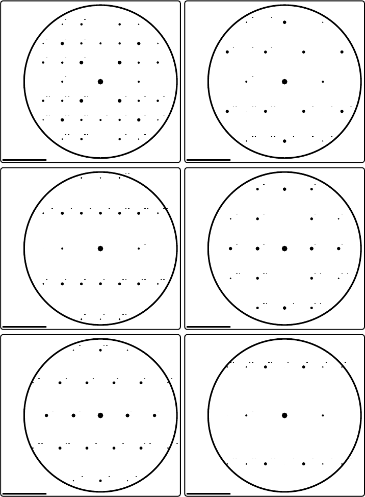
Example output from the zap.f90 program is shown in Fig. 3.35; the program

draws six patterns per page, in this case the lowest-order zone axis patterns for

rutile (TiO

, 200 kV, L = 1600 mm). The computed patterns show reﬂections as

solid circles with a diameter related to the calculated intensity I

. The program

implements two different intensity scales.

Logarithmic intensity scale. This scale computes the radius r

to be used for a given

diffraction spot using the following relation [GW87]:

= c

log(1 + c

), (3.72)

with c

and c

constants. The zap.f90 program uses c

= 1.27 mm (=

in) and c

= 0.1.

Exponential intensity scale. An alternative intensity scale compresses the entire range

of intensities by suppressing the higher intensities and increasing the lowest intensities.

210 The transmission electron microscope

Zone axis [ 0 0 1]

Multiplicity 2

1 1 0

110

1 10

2 00 200

020

120

210

2 1 0 210

1 20 120

1 2 0

2 10

2 2 0

220

2 20

130

310

3 1 0 310

1 30 130

1 3 0

3 10

230

320

2 30

3 20

230

2 3 0

3 2 0

Zone axis [ 1 0 0]

Multiplicity 4

011

011 011

011

020020

021

021021

021

002

012

012012

012

031 031

031031

022022

022 022

Zone axis [ 1 0 1]

Multiplicity 8

101

1 01

020 020

111 111

1 1 11 11 12 1

121

1 21

121131

1 3 11 31

131

202

2 02

212212

2 12 2 1 2

Zone axis [ 1 1 0]

Multiplicity 4

110 1 10

1 11

111 1 11

111

220 2 20

002

2 21

221

2 21

1 12

112

Zone axis [ 1 1 1]

Multiplicity 8

110 1 10

101 011

011 1 01 211

211 121

121

2 20220

1 1 2

112202

022 2 02

022

3 21231

321 231

Zone axis [ 1 0 2]

Multiplicity 8

020 020

201

2 01

211

2 112 1 1

211 221221

2 2 1 2 212 3 1 231

231231

Fig. 3.35. Example output of the zap.f90 program for the lowest-order zone axis patterns

of rutile (TiO

, 200 kV, L = 1600 mm). The ﬁgure has been reduced to 70% to ﬁt on the

page.

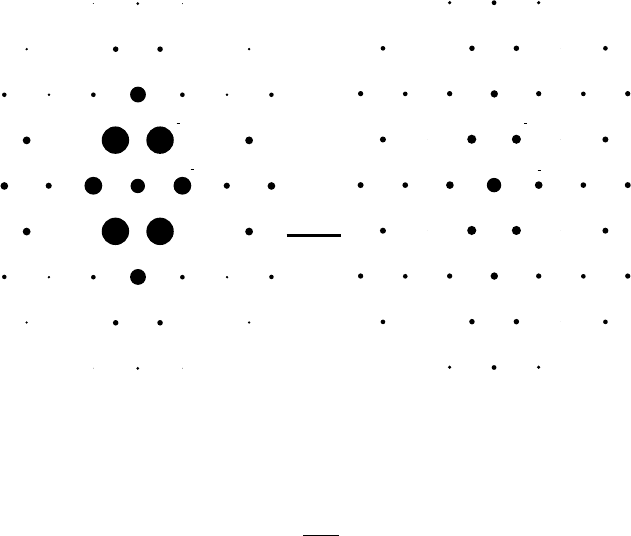
3.9 The specimen stage 211

110

5 nm

-1

110

(a) (b)

Fig. 3.36. [11.3] zone axis pattern for hexagonal Ti (200 kV, L = 800 mm): (a) logarithmic

and (b) exponential intensity scaling.

This can be accomplished by a scaling relation of the following type:

= c



max



, (3.73)

where I

max

is the maximum intensity. The zap.f90 program uses c

= 1.27 mm and

= 0.2.

A comparison of the two intensity scales is shown in Fig. 3.36 for the [11.3] zone

axis pattern of hexagonal Ti, for a microscope acceleration voltage of 200 kV

and camera length L = 800 mm. Figure 3.36(a) uses logarithmic intensity scaling

and Fig. 3.36(b) shows the exponential scaling. For comparison with experimental

diffraction patterns the exponential scaling often provides better visual agreement.

3.9.5 Higher-order Laue zones

3.9.5.1 Deﬁnition and examples

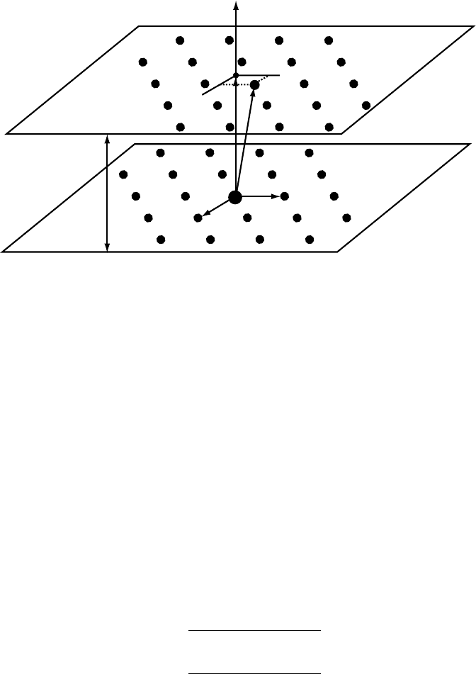
The reciprocal lattice is a three-dimensional lattice and in any given zone axis pattern

we observe a nearly planar section through this lattice. The reciprocal lattice planes

parallel to the plane imaged in a zone axis pattern (Fig. 3.37) also intersect the

Ewald sphere, but at a rather large distance from the origin of reciprocal space. We

recall from Chapter 1 that the set of reciprocal lattice points belonging to a zone

axis pattern can be described by means of the zone equation:

g · t = hu + kv + (it) + lw = 0, (3.74)

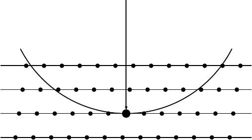
212 The transmission electron microscope

ZOLZZOLZ

FOLZFOLZ

SOLZSOLZ

ESES

Fig. 3.37. Schematic illustration of the geometry of higher-order Laue zones or HOLZ.

where the term it only occurs for the 4-index hexagonal case. This set of reciprocal

lattice points is also known as the zero-order Laue zone,orZOLZ.

Reciprocal lattice planes parallel to the ZOLZ satisfy the equation

hu + kv + (it) + lw = N , (3.75)

where N is a non-zero integer. The exact values of N depend on the zone axis

direction t. The integer N effectively numbers the reciprocal lattice planes, which

are then known as the higher-order Laue zones,orHOLZ. The lowest non-zero

value for N for which reﬂections are allowed corresponds to the ﬁrst-order Laue

zone (FOLZ), the next value to the second-order Laue zone (SOLZ), and so on.

†

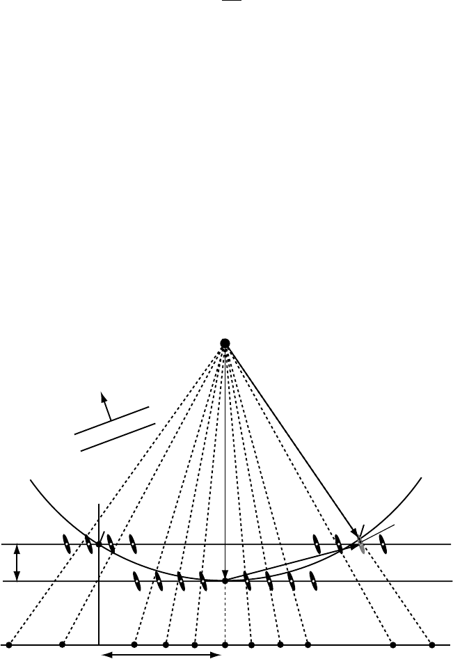
3.9.5.2 Simulation of HOLZ diffraction patterns

The simulation of electron diffraction patterns that contain reﬂections from HOLZ

layers is not very difﬁcult and only requires a careful deﬁnition of an appropriate

reference frame. Consider a zone axis diffraction pattern, recorded with the beam

along the t = [uvw] direction. We can always select two short reciprocal lattice

vectors as basis vectors of the ZOLZ, say g

and g

(see Fig. 3.38). The vectors are

selected so that the reference frame is right-handed, i.e. g

× g

 t. The third basis

vector g

is selected along t so that its length is equal to the distance between the

plane formed by g

and g

and the next plane (i.e. the plane for which N = 1in

equation 3.75). Because of the duality between real space and reciprocal space we

know that this distance is given by the inverse of the length of t or 1/|t|≡H.We

will use the vectors g

(i = 1,...,3) as basis vectors for all computations involving

HOLZ reﬂections, including Kikuchi lines and HOLZ line computations discussed

†

It is possible for entire planes in reciprocal space to consist of forbidden reﬂections. In such a case there may

be no reﬂections for N = 1, while the ﬁrst ring of visible reﬂections has N = 2. This ring is still known as

the ﬁrst-order Laue zone. In other words, the value of N is not necessarily equal to the order of the HOLZ

layer [Ead90].

3.9 The specimen stage 213

FOLZ

ZOLZ

[uvw]

hu+kv+lw = 1

hu+kv+lw = 0

Fig. 3.38. Reference frame used for HOLZ computations.

in Chapter 9. A numerical procedure for determining the new reference frame will

be introduced in Chapter 7.

In some crystal structures, the reciprocal vector g

will be a reciprocal lattice

vector (meaning that it can be written as an integer linear combination of the vectors

∗

). In other structures, or for other zone axes, the vector g

will not be a reciprocal

lattice vector. In such cases the reﬂections on the plane N = 1 will be shifted with

respect to those of the ZOLZ. We will take the vector G to be the shortest reciprocal

lattice vector of the N = 1 plane (Fig. 3.38). Any vector in the FOLZ can then be

written as the sum of a vector in the HOLZ and G. More generally, any reciprocal

lattice vector h can be written as

h = (n

+ NG

+ (n

+ NG

+ N g

, (3.76)

where n

and n

are integers, and G

are the components of G along the vectors g

It is not difﬁcult (exercise) to show that

G · g

− G · g

− γ

;

G · g

− G · g

− γ

with γ

= g

· g

The projection of the vector G onto the ZOLZ plane can also be found using a

method proposed by Jackson [Jac87]. If t

∗

represents the reciprocal space vector

corresponding to t, i.e. t

∗

= t

(see Chapter 1), then the vector connecting the

214 The transmission electron microscope

ZOLZ to the N th HOLZ layer is given by

⊥

∗

HN.

Subtracting this vector from the vector NG results in the projection N g

, i.e.

N g

= N G − G

⊥

This vector clearly lies in the ZOLZ plane. It is then simply a matter of express-

ing the vector g

with respect to the basis vectors g

and g

to recover the compo-

nents G

Next, we must determine where a diffracted beam corresponding to a HOLZ

reﬂection will intersect the viewing screen. Consider Fig. 3.39: the reciprocal lattice

points are represented by relrods parallel to the foil normal F. A diffracted beam

corresponding to the reﬂection g will intersect the ZOLZ in a point on the line k



CQ. The reader should note that the foil normal F may have a component out of the

plane of the drawing, so that the scattered vector k



need not lie in the plane formed

ZOLZ

FOLZ

Observation scr

een

Fig. 3.39. Intersection of FOLZ relrods with the Ewald sphere result in a diffracted beam

in the direction k



= k

+ g + s

3.9 The specimen stage 215

by k

and g. The coordinates of the point Q can be found from the vector sum:



= k

+ g + s.

These three vectors can be expressed in the g

reference frame:

g = (n

+ NG

+ (n

+ NG

+ N g

;

=−

λH

;

s = s

+ F

where F

are the components of the unit vector

F with respect to g

. Combining

these equations we ﬁnd for k



= (n

+ NG

+ s

+ (n

+ NG

+ s



N −

λH

+ s



If we scale this vector so that the point Q moves to P along the line CQ, then the

ZOLZ coordinates of the point P can be found by making the g

component of k



equal to −1/λH . The resulting ZOLZ position vector is then given by

1 − λH (N + s

)



i=1

+ NG

+ s

. (3.77)

This vector can then be scaled by the camera constant λL to ﬁnd the position

of the HOLZ reﬂection g on the viewing screen. Equation (3.77) is valid for all

HOLZ reﬂections, including the ZOLZ reﬂections, and takes into account the foil

normal and the curvature of the Ewald sphere. We leave it to the reader to derive

an expression for g

when the incident beam direction is tilted away from the zone

axis t, so that k

acquires components along g

and g

The point R in Fig. 3.39 indicates the intersection of the Ewald sphere with the

HOLZ layer. The intersection forms a ring, known as the HOLZ ring. The radius

of the nth HOLZ ring can be computed from the equation of the Ewald sphere

as follows:

(

− H

, (3.78)

where H

= nH. The term H

is often small and can be ignored. This radius R

can be measured from an experimental electron diffraction pattern. The procedure

will be illustrated in Chapter 9.

In Chapters 5–7, we will describe how the intensity of a diffracted beam depends

on the distance of the reciprocal lattice point to the Ewald sphere, i.e. the excitation

error s

. In the simplest approximation, the intensity I

of a reﬂection g has a sinc

216 The transmission electron microscope

dependence on the excitation error, i.e.

→ I



sin(π z

)

π z



= I

sinc

(π z

where z

is the foil thickness. This follows from the so-called kinematic theory

introduced in Chapter 6; it can also be derived from the expression for the relrod

intensity in Chapter 2 (Section 2.6.3). For each reﬂection closer to the Ewald sphere

than a preset threshold distance, s

max

, we compute the scaled intensity and use it

to determine the radius of the circle representing the reﬂection in a drawing of the

diffraction pattern.

Pseudo code

PC-13 outlines the major computational steps of the program

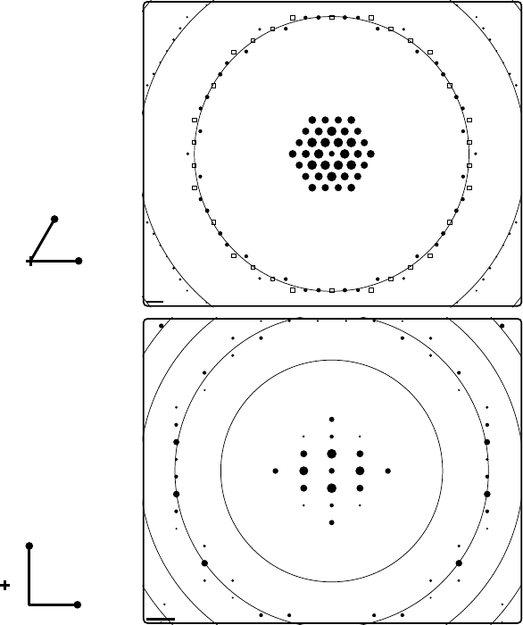
HOLZDP.f90; example output from this program is shown in Fig. 3.40 for the [00.1]

zone axis pattern of Ti and the [112] pattern of GaAs. We will return to HOLZ-

related computations and observations in Chapters 7 and 9.

Pseudo Code PC-13 Zone axis diffraction patterns with HOLZ reﬂections.

Input: PC-2 , PC-3

Output: HOLZ zone axis patterns in PostScript format

ask for microscope voltage and camera length

for each incident beam direction do

determine g

basis vectors and G

get foil normal F and Laue center

compute radii R

of HOLZ circles

determine contributing reﬂections for ZOLZ

plot ZOLZ pattern

for every HOLZ layer do

determine contributing reﬂections

plot HOLZ pattern

end for

label selected reﬂections

end for

3.10 The magniﬁcation stage: post-specimen lenses

The post-specimen part of the objective lens ﬁeld is used to magnify the image,

typically by a factor of 30–50 times. Most microscopes have at least three other

lenses following the objective lens. They are usually known as (from top to bottom)

the diffraction lens (DL), the intermediate lens (IL), and the projector lens (PL). A

3.10 The magniﬁcation stage: post-specimen lenses 217

Zone axis [ 0 0 . 1]

HOLZ radii [nm

-1

]

1 41.2211

2 58.2172

3 71.2051

( 1 0 . 0)

( 0 1 . 0)

Zone axis [ 1 1 2]

HOLZ radii [nm

-1

]

1 19.7415

2 27.9000

3 34.1475

4 39.4037

( 1

( 1 1

GaAs

-1)

-1 0)

Fig. 3.40. Simulated zone axis patterns with HOLZ reﬂections for Ti and GaAs. The HOLZ

ring radii are indicated. The small + sign indicates the shift vector G of the FOLZ with

respect to the HOLZ layer.

cross-sectional view of the imaging stage of the JEOL 120CX microscope is shown

in Fig. 3.32(b). In the following paragraphs we will add these lenses one at a time,

to make clear why they are all needed.

If the objective lens were the only imaging lens present, then the situation would

be rather simple. Since both the specimen and the observation screen have a ﬁxed

location, the object and image distances are ﬁxed, and this in turn determines

the focal length (and magniﬁcation) of the objective lens (see Section 3.4.6). The

objective lens current can be varied to bring the image plane into exact coincidence

with the screen (this is known as focusing), at which point everything is ﬁxed.

To obtain a system with a variable magniﬁcation we must add a second lens, the

projector lens PL.