Graef M. Introduction to conventional transmission electron microscopy

Подождите немного. Документ загружается.

218 The transmission electron microscope

specimen

screen

(fixed)

specimen

screen

back focal plane

(fixed)

selected area plane

(fixed)

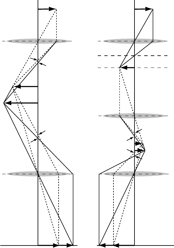
Fig. 3.41. (a) Two-lens system consisting of objective OL and projector PL lenses. Ray

diagrams for two different overall magniﬁcations are shown, and the locations of the focal

points are arrowed; (b) three-lens system with ﬁxed OL current. Again two different overall

magniﬁcations are shown.

The ray diagram in Fig. 3.41(a) shows how two images 1 and 2 with different

magniﬁcation can be generated by the two lenses OL and PL. The ray diagram is

constructed based on Fig. 3.9, and for simplicity we have made the two principal

planes Po and Pi coincide (this is known as the thin-lens approximation); while

this is not necessarily a realistic approximation, it does simplify the ray diagrams

substantially and it is sufﬁcient to illustrate how sets of lenses work.

3.10 The magniﬁcation stage: post-specimen lenses 219

We will use ray pairs 1–3 or 2–3 (in the notation of Fig. 3.9) to obtain the location

of image and object planes in Fig. 3.41. Two sets of rays are shown (solid and dashed

lines) for two different excitations of the lenses. When the OL current is decreased,

the image focal length increases (the focal points are arrowed) and the image plane

moves down the optical axis. This plane then becomes the object plane for the PL

and two images with different overall magniﬁcations are obtained. The PL current

must be increased to bring the object focal point (arrowed) closer to the center of

the lens. The overall magniﬁcation is then the product of the magniﬁcations of each

lens, as can be veriﬁed easily by direct multiplication of the two transfer matrices

(Section 3.4.6).

Although we have reached our goal of a variable magniﬁcation system, there

are several drawbacks to this setup. First of all, it is actually desirable to have

an objective lens with a ﬁxed current: for high-magniﬁcation observations small

variations in the lens temperature can cause large specimen drifts, so large current

changes in the objective lens must be avoided. In most observation modes, we use

the objective lens at a given current, and focusing is carried out by small adjustments

of this current (changes of a few tenths of a percent). There is another advantage

to having a ﬁxed OL current: the image plane conjugate to the specimen has a

ﬁxed location along the optical axis. This plane is rather important for conventional

TEM work, and it is known as the selected area or SA plane. From here on, we will

assume that the OL current is such that the SA plane, a plane ﬁxed by the location

of the SA aperture, is conjugate to the specimen plane. This also ﬁxes the back

focal plane and the diffraction aperture.

Since the ﬁxed OL current also ﬁxes the PL current for which the object plane is

conjugate to the screen, we must add a third lens (intermediate lens, IL) to regain

control over the magniﬁcation of the system. Adding a third lens to a system with

a ﬁxed OL current has the same effect as adding the projector lens to the variable

OL: a variable magniﬁcation is again obtained, as shown in the ray diagram of

Fig. 3.41(b). The SA plane is the object plane for the intermediate lens, while the

observation screen is the image plane for the projector lens. Changing the current

in both IL and PL creates a variable magniﬁcation system.

There is still one signiﬁcant drawback to a three-lens system: a given magni-

ﬁcation can only be reached in one way. To reduce the combined effects of the

lens aberrations it is desirable to have more than one way to create a given mag-

niﬁcation, so that the method with the lowest overall aberration can be used. This

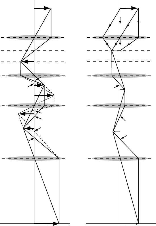
can be obtained by adding yet another lens, the diffraction lens DL. As shown in

Fig. 3.42(a), several combinations of IL and PL lens currents can be used to obtain

the same overall magniﬁcation. We can also vary the current in the DL to have

the OL back focal plane as the object plane, and hence a magniﬁed image of the

electron diffraction pattern can be obtained, as shown in Fig. 3.42(b).

220 The transmission electron microscope

specimen

screen

1=2

back focal plane

(fixed)

selected area plane

(fixed)

specimen

screen

back focal plane

(fixed)

selected area plane

(fixed)

(a) (b)

Fig. 3.42. (a) Four-lens system. Two ray diagrams with the same overall magniﬁcation

are shown, illustrating that the same magniﬁcation can be obtained in more than one way.

(b) Four-lens system with the OL back focal plane as object plane for the diffraction lens

DL; this produces a magniﬁed diffraction pattern on the viewing screen.

Since the focal length of a magnetic lens, and, hence, its magniﬁcation, depend

on the electron energy, and the SA plane is a ﬁxed plane, it is clear that a change

in the microscope acceleration voltage must be accompanied by a change in lens

currents, to maintain the appropriate relations between the ﬁxed conjugate planes.

Electron microscopes, therefore, have several preset lens currents for a number of

acceleration voltages.

3.11 Electron detectors 221

Not all lenses are excited for all observation conditions. Whenever a lens switches

on or off, the microscope operator will observe an inversion of the image, since a

cross-over is added to or removed from the beam path. Some microscopes have an

objective minilens, a weak lens located between the OL and DL; this lens is used for

low-magniﬁcation observations, for which the main OL is switched off completely.

In other microscopes there is a second projector lens to compensate for the fact

that the electron beam must go through a narrow differential pumping aperture just

below the IL. We can discern a general rule of thumb: for every new ﬁxed cross-

over an additional lens must be added to keep the ﬂexibility of the system the same.

Finally, by carefully matching the lens currents for all imaging lenses in the column

one can compensate for the image rotation caused by the Lorentz force and obtain a

column with nearly zero overall image rotation over the entire magniﬁcation range.

3.11 Electron detectors

3.11.1 General detector characteristics

A good electron detector should have the following characteristics:

sensitivity down to single electrons;

a linear relation between the incident intensity and the detector signal for a wide range of

intensities;

high spatial resolution;

low noise level;

high detector readout speed or frequency;

reproducibility.

Additional characteristics, such as ease of use, lifetime, and cost, may also be

important. In the following subsections, we will discuss the discreteness of digital

images and factors affecting the intensity measured by a detector. We will conclude

this chapter with a brief description of the viewing screen, photographic emulsions,

and charge-coupled device (CCD) cameras.

3.11.1.1 Detector pixel size

We will assume that we can deﬁne a detector pixel size, i.e. the size of the smallest

region (usually a square) that contains a readable signal. For a charge-coupled

device camera the pixel size is set by the physical dimensions of the sensitive area,

typically around 25 × 25 = 625

µm

. For a photographic negative the pixel size

is of the order of the silver halide grain size. After digitization of a photographic

negative the pixel size would be determined by the scanning resolution. Digitization

at 1200 “dots-per-inch” or dpi is equivalent to a pixel size of 21

µm, similar to that

of a CCD camera [Ead96].

222 The transmission electron microscope

Since electronic images are always discrete images, sampled on a square grid of

pixels, we must take a closer look at the details of sampling; in particular, we must

ask the question: when is a sampled image a reliable representation of the actual

image?

Consider a continuous function f (x) with Fourier transform f (q), i.e.

f (q) = F

[

f (x)

]

+∞

−∞

f (x)e

−2πiqx

dx.

The function f (x) can be sampled with a sampling interval δ, so that we obtain a

series of discrete values

≡ f (iδ), i =−∞,... ,−1, 0, 1,... ,+∞.

The inverse of the sampling interval is known as the sampling rate. We deﬁne the

Nyquist critical frequency as half of the sampling rate:

≡

2δ

. (3.79)

The sampling theorem then states the following [PFTV89]: if a continuous function

f (x), sampled at an interval δ, is band-width limited to frequencies smaller than

(i.e. f (q) = 0 for all frequencies q > q

), then that function f (x) is completely

determined by the samples f

. The value f (x) at any point in between two sampling

points may be determined using the following interpolation relation:

f (x) =

+∞



i=−∞

sinc[2πq

(x − iδ)]. (3.80)

If the sampling interval δ is too large, so that f (q) is non-zero for q > q

, then

the sampling theorem fails, and the sampled function f

will not be a faithful

representation of the actual function f (x). If the function f (x) varies on a length

scale smaller than δ, then the spatial frequencies corresponding to this length scale

will not be properly represented in the Fourier transform, and the low-frequency

Fourier coefﬁcients will contain information on the high-frequency behavior of the

function. This phenomenon is known as aliasing.

The main conclusion from this brief discussion of sampling is then that a digital

representation of a continuous signal should have a sampling rate that is at least

twice that needed to represent the smallest details of interest in the signal. Since

the detector pixel size often effectively sets the sampling interval δ, this means

that images must be acquired at the proper microscope magniﬁcation. In numerical

computations with discrete images, it is often convenient to explicitly set all function

values in the direct discrete Fourier transform (DDFT) of the image to zero for

spatial frequencies beyond the Nyquist limit q

3.11 Electron detectors 223

3.11.1.2 Intensity levels for individual pixels

An ideal detector would be capable of detecting single electrons. Each pixel (i, j)

in the image generated by such a detector would therefore contain an intensity

I (i, j) equal to the number of electrons that reached the pixel (i, j ). For “real”

detectors, the situation is somewhat more complicated because: (a) the signal from

an individual electron may be spread over multiple pixels; (b) not all electrons may

be detected; and (c) the inherent noise level in the detector electronics may place a

lower limit on the number of electrons detected.

The quality of a detector can be quantiﬁed by the so-called detective quantum

efﬁciency or DQE. Rose [Ros46] has deﬁned the DQE as the squared ratio of the

signal-to-noise ratio of the detector output to the signal-to-noise ratio of the input

signal, or

DQE ≡

(

S/N

)

output

(

S/N

)

input

. (3.81)

The DQE varies from 0 (only noise as the detector output) to 1 (the detector adds

no noise to the signal). The signal-to-noise ratio can be deﬁned as the mean image

intensity

I divided by the standard deviation of the intensity σ (I ):

S/N =

σ (I )

(3.82)

with

I =



i=1



j=1

I (i, j);

σ (I ) =

MN − 1



i=1



j=1

I (i, j) −



1/2

The square of the standard deviation is known as the variance var(I ).

The DQE deﬁned above implicitly assumes that a single electron can only cause

a signal in a single pixel. In reality, a single electron may cause a signal in a small

neighborhood of pixels. This “spreading” of the signal is mathematically described

by the point spread function T . The signal I

measured by the detector is then the

convolution of the actual incident intensity, I (i, j), and the point spread function

T (i, j ), or

(i, j) = I (i, j ) ⊗ T (i, j). (3.83)

It is often convenient to express this relation in Fourier space as

F[I

(i, j)] ≡ I

(µ, ν) = I (µ, ν)T (µ, ν),

224 The transmission electron microscope

where T (µ, ν) = F[T (i, j)] is the modulation transfer function or MTF, and the

components (µ, ν) indicate the spatial frequency. The point spread function concept

is valid for both photographic and electronic detectors, and we will make extensive

use of this concept in Chapter 10. Note that if T (µ, ν) is known and non-zero for all

spatial frequencies, then the incident intensity I can be retrieved from the detected

intensity I

by a simple division in Fourier space:

I (µ, ν) =

(µ, ν)

T (µ, ν)

Fortunately, the MTF for photographic ﬁlm and for CCD cameras does not contain

any zero-crossings for frequencies up to q

, and therefore this type of deconvolution

is possible, assuming I

(µ, ν) has been zeroed for spatial frequencies beyond q

As a consequence of the frequency-dependent response of the detector system, the

DQE also becomes frequency dependent, i.e. DQE(µ, ν) [dRMK93].

In the absence of an incident signal, a detector would ideally produce a zero-

intensity signal. In practice, there will be a small signal due to noise in the detector

electronics, noise generated by cosmic radiation hitting the active areas of the

detector, and so on. An image acquired without any incident intensity is known as a

dark image, D(i, j), or a background image. The dark image should be subtracted

from each acquired image, since it is common to all images. A dark image should

be acquired with the same exposure time and other recording settings as the actual

image.

The sensitivity of pixels may vary across the detector. In the case of a charge-

coupled device camera the incident electrons are typically converted to light by

a scintillator layer, and subsequently this light signal travels through a ﬁber-optic

connector to the CCD surface. The internal structure of this ﬁber-optic connection

creates spatial variations of the detected signal, even for a homogeneous incident

illumination. This sensitivity must be removed from the image before any image

processing may be carried out. This is accomplished by the acquisition of a gain

reference image, G(i, j), using uniform illumination. Correction of the sensitivity

variations of individual pixels is known as gain normalization.

The true incident intensity I (i, j) can be derived from the detector signal I

(i, j)

by means of the following operations:

I = F

−1

−D

G−D

(G − D)

F[T ]

, (3.84)

where the overbar denotes the average over the entire image. The ﬁrst operation

(background subtraction and gain normalization) can be performed in real time,

since the inverse of the gain reference image can be stored in memory. Deconvo-

lution of the point spread function is slightly more time consuming, and is usually

3.11 Electron detectors 225

not performed in real time. Note that this procedure is quite general and applies to

all detectors with a non-zero modulation transfer function T (µ, ν).

The intensity I

(i, j) has a range from 0 to a maximum intensity I

max

, which

depends on how many electrons a pixel can detect before saturation occurs. For

electronic detectors, this is given by the number of bits per pixel; if a detector uses

12 bits per pixel, then the range of detectable intensities is from 0 to 2

− 1 or 4096

gray levels. This interval is known as the dynamic range of the detector. It would

appear that a 12-bit detector would be able to distinguish 4096 incident intensity

levels. However, since the arrival of electrons at the detector is itself a statistical

process, there is no statistically signiﬁcant difference between, say, 4000 counts and

4001 counts. In fact, the standard deviation of the number N of electrons which

reaches a detector element obeys Poisson statistics, and is given by

√

N . This means

that for N = 4000 the standard deviation is about 63, so that all pixels with counts

between N = 3937 and N = 4063 are statistically equivalent. The random arrival

of electrons is known as shot noise or Poisson noise. For a detailed discussion of

shot noise and related topics we refer the interested reader to [Spe88, Section 6.8].

The human eye itself has a non-linear response to incident intensity. Physiological

measurements indicate that the “electrical output” of the human eye is proportional

to the logarithm of the stimulus (Weber–Fechner’s law). This is reﬂected in the

magnitude scale used for the apparent brightness of stars; the original magnitude

scale covers the range from 1 (brightest) to 6 (faintest), which corresponds to a factor

of 100 in absolute intensity change. Therefore the linear magnitude scale actually

corresponds to an exponential scale with base 2.512, since (2.512)

= 100. As a

direct consequence of its logarithmic response, the human eye can only distinguish

between a limited number of gray values in an image, typically on the order of 30

different gray levels. The eye is, therefore, not a very good instrument to compare

quantitatively the intensity distributions of experimental and simulated images.

After the “true” image intensity has been determined by means of equation (3.84),

other image processing operations may be performed on I (i, j). Typical operations

are high-pass and low-pass ﬁltering, edge enhancement, Fourier analysis, smooth-

ing, and so on. The literature on image processing is extensive, and the reader is

encouraged to consult The Image Processing Handbook, by J.C. Russ [Rus92],

for further information. The ﬁeld of image algebra formalizes the ways in which

images can be manipulated. For an introduction to image algebra, the reader is

referred to Chapters 70–76 in [HK94].

The last step in any image processing procedure is always the visualization of the

ﬁnal image on a computer screen or in printed form. Grayscale images are typically

represented on a linear 8-bit intensity scale, so that there are 256 output gray levels

available. Image intensities need not be mapped linearly into the available gray

levels. A commonly used mapping is based on equation (3.73) on page 211, with

226 The transmission electron microscope

= 255 and c

= γ (in some image processing systems, c

is set equal to 1/γ ).

A gamma-factor of γ = 1 produces a linear intensity mapping between 0 and 255.

For values of γ>1 the lowest intensities are compressed into fewer gray levels,

while for γ<1 the higher intensity values are compressed. This type of non-linear

scaling enhances the image contrast; the percentage contrast between two pixels is

deﬁned by

%C =

− I

+ I

× 100. (3.85)

The shot noise in an image along with the saturation value of each pixel deter-

mine the smallest percentage contrast that can be obtained. If a pixel has I counts

and the neighboring pixel has I + dI counts, then the percentage contrast is given

by [Ead96]:

%C =

100

2I /dI + 1

;

100

√

I + 1

≈

100

√

We have used the fact that two pixels have a statistically different intensity only when

dI > 2

√

I . For large values of I the last expression provides a good approximation.

For I = 10 000 the lowest percentage contrast that is statistically meaningful would

be around 1.0%.

The average intensity of the image,

I , is the image brightness. Image brightness

can be changed by a mapping of the form

display

= c

min

+ (c

max

− c

min

)



max



If c

max

is smaller than 255, the overall image brightness decreases; if c

min

is larger

than 0, then the image brightness increases. It is obvious that brightness is changed

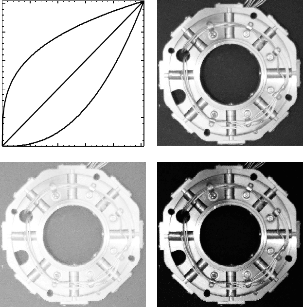
at the expense of the number of available display gray levels. Figure 3.43(a) shows

two different contrast scaling functions for γ = 0.3 and 2.5 for the display in-

tensity range [0, 255]. The effect of both scalings on a reference image is shown

in Figs 3.43(c) and (d), which represent gamma-scaled versions of the image in

Fig. 3.43(b).

The reader should be warned that with modern image processing packages it is

all too easy and often quite tempting to enhance experimental images, by changing

the contrast or by sharpening the details. If images derived from an experiment

(i.e. after application of equation 3.84 to the detected images I

(i, j)) are to be

used for comparison with numerically simulated images, no image altering oper-

ations should be performed before the comparison has been completed! If image

3.11 Electron detectors 227

100

150

200

250

0 50 100 150 200 250

γ = 2.5

γ = 0.3

γ = 1.0

(a)

(b)

γ = 2.5

γ = 0.3

γ = 1.0

Fig. 3.43. (a) Gamma correction curves; (b) reference image (condensor stigmator of JEOL

120CX); (c) gamma-scaled image for γ = 0.3; (d) gamma-scaled image for γ = 2.5.

modiﬁcations or enhancements are made (smoothing, ﬁltering of noise, etc.), then

this should be stated explicitly in the ﬁgure caption or text accompanying the ﬁgure.

3.11.2 Viewing screen

The ﬁnal stage in the microscope detects the electrons and forms an observable

image. This is routinely accomplished with a phosphor (or ZnS) viewing screen,

where the incident electrons excite outer-shell electrons and “green” photons

†

are

emitted when these fall back to their low-energy states. With high-intensity electron

beams, some “burn-in” can occur if the beam is focused on one point for too long.

Viewing screens are therefore replaced every couple of years. The resolution of a

†

The human eye is most sensitive in the green portion of the visible electromagnetic spectrum, and therefore the

screen phosphor is designed to emit most strongly in this frequency range.