Griffiths D. Head First Statistics

Подождите немного. Документ загружается.

you are here 4 571

the χ

distribution

The χ

test assesses difference

There’s a new sort of probability distribution that does exactly what we want;

it’s called the χ

distribution. χ is pronounced “kye”, and it’s the uppercase

Greek letter chi. It uses a test statistic to look at the difference between what

we expect to get and what we actually get, and then returns the probability of

getting observed frequencies as extreme.

Let’s start with the test statistic. To find the test statistic, first make a table

featuring the observed and expected frequencies for your problem. When

you’ve done that, use your observed and expected frequencies to compute the

following statistic, where O stands for the observed frequency, and E for the

expected frequency:

Use the table of observed and expected frequencies you just

worked out on the previous page for Fat Dan’s slot machines to

compute the test statistic. What result do you get?

What do you think a low value tells you? What about a high value?

In other words, for each probability in the probability distribution, you take

the difference between the frequency you expect and the frequency you

actually get. You square the result, divide by the expected frequency, and

then add all of these results up together.

So what’s the test statistic for the slot machine problem?

O refers to the observed frequency, while

E refers to the expected frequency.

(O - E)

572 Chapter 14

So at what point does Χ

become so large that it’s significant? We need to

figure out when we can fairly certain that something’s going on with the slot

machines that’s beyond what could reasonably happen by chance.

To find this out, we need to look at the χ

distribution.

Use the table of observed and expected frequencies you just

worked out on the previous page for Fat Dan’s slot machines to

compute the test statistic. What result do you get?

What do you think a low value tells you? What about a high value?

So what does the test statistic represent?

The test statistic Χ

gives a way of measuring the difference between the

frequencies we observe and the frequencies we expect. The smaller the value

of Χ

, the smaller the difference overall between the observed and expected

frequencies.

You divide by E, the expected frequency, as this makes the result proportional

to the expected frequency.

The smaller the differences between O

and E, the smaller X

is.

Dividing by E makes the difference

proportional to the expected frequency.

= (965 - 977)

/977 + (10 - 8)

/8 + (9 - 8)

/8 + (9 - 6)

/6 + (7 - 1)

= (-12)

/977 + 2

/8 + 1

/8 + 3

/6 + 6

= 144/977 + 4/8 + 1/8 + 9/6 + 36

= 0.147 + 0.5 + 0.125 + 1.5 + 36

= 38.272

If the value of X

is low, then this means there’s a less significant difference between the observed and expected

frequencies. The higher X

is, the more significant the differences become.

another sharpen solution

(O - E)

you are here 4 573

the χ

distribution

Two main uses of the χ

distribution

The χ

probability distribution specializes in detecting when the results you

get are significantly different from the results you expect. The probability

distribution does this using the Χ

test statistic you saw earlier.

The χ

distribution has two key purposes.

First of all, it’s used to test goodness of fit. This means that you can use

it to test how well a given set of data fits a specified distribution. As an

example, we can use it to test how well the observed frequencies for the slot

machine winnings fits the distribution we expect.

Another use of the χ

distribution is to test the independence of two

variables. It’s a way of checking whether there’s some sort of association.

The χ

distribution takes one parameter, the Greek letter ν, pronounced

“new.” Let’s take a look at the effect that ν has on the shape of the

probability distribution.

A shorthand way of saying that you’re using the test statistic Χ

with the

distribution that has a particular value of ν is

~ χ

(ν)

follows a χ

distribution with a given value of ν.

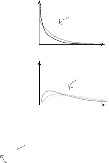
When ν is 1 or 2

When ν has a value of 1 or 2, the shape of the χ

distribution

follows a smooth curve, starting off high and getting lower. It’s

shape is like a reverse J. The probability of getting low values of

the test statistic Χ

is much higher than getting high values. In

other words, observed frequencies are likely to be close to the

frequency you expect.

When ν is greater than 2

When ν has a value that’s greater than 2, the shape of the χ

distribution changes. It starts off low, gets larger, and then

decreases again as Χ

increases. The shape is positively skewed,

but when ν is large, it’s approximately normal.

It’s like an X, but curvier.

The χ

distribution has this

sort of shape if ν is 1 or 2.

It has this sort of shape if ν

is greater than 2. The larger

ν becomes, the more normal

the χ

distribution gets.

574 Chapter 14

ν = (number of classes) - (number of restrictions)

ν = 5 – 1

= 4

ν represents degrees of freedom

You’ve seen how the shape of the χ

distribution depends on the value of ν, but

how do we find what ν is?

ν is the number of degrees of freedom. It’s the number of independent

variables used to calculate the test statistic Χ

, or the number of independent

pieces of information. Let’s see what this means in practice.

Here’s another look at the table of observed and expected frequencies for the

slot machines:

The number of degrees of freedom is the number of expected frequencies we

have to calculate, taking into account any restrictions we have upon us.

In order to calculate the test statistic Χ

, we had to calculate all of the expected

frequencies. This meant that we had to calculate five expected frequencies.

While calculating this, we had one thing we had to bear in mind: the total

expected frequency and the total observed frequency had to add up to the same

amount. In other words, we had one restriction on us in our calculations.

So what’s ν?

To calculate ν, we take the number of pieces of information we calculated, and

subtract the number of restrictions. To figure out the test statistic Χ

, we had to

calculate five separate pieces of information, with 1 restriction. This means that

the number of degrees of freedom is given by

In general,

x Observed frequency Expected frequency

-2

965 977

10 8

9 8

9 6

7 1

Another way of looking at this is that we had to calculate four of the expected

frequencies using the probability distribution. We could work out the final

frequency by looking at what the total expected frequency should be.

degrees of freedom

you are here 4 575

the χ

distribution

Tail probability α

.25 .20 .15 .10 .05 .025 .02 .01 .005 .0025 .001

1 1.32 1.64 2.07 2.71 3.84 5.02 5.41 6.63 7.88 9.14 10.83

2 2.77 3.22 3.79 4.61 5.99 7.38 7.82 9.21 10.60 11.98 13.82

3 4.11 4.64 5.32 6.25 7.81 9.35 9.84 11.34 12.84 14.32 16.27

4 5.39 5.99 6.74 7.78 9.49 11.14 11.67 13.28 14.86 16.42 18.47

5 6.63 7.29 8.12 9.24 11.07 12.83 13.39 15.09 16.75 18.39 20.51

6 7.84 8.56 9.45 10.64 12.59 14.45 15.03 16.81 18.55 20.25 22.46

7 9.04 9.80 10.75 12.02 14.07 16.01 16.62 18.48 20.28 22.04 24.32

8 10.22 11.03 12.03 13.36 15.51 17.53 18.17 20.09 21.95 23.77 26.12

9 11.39 12.24 13.29 14.68 16.92 19.02 19.68 21.67 23.59 25.46 27.88

What’s the significance?

So how can we use the χ

distribution to say how significant the

discrepancy is between the observed and expected frequencies? As

with other hypothesis tests, it all depends on the level of significance.

When you conduct a test using the χ

distribution, you conduct a one-

tailed test using the upper tail of the distribution as your critical region.

This way, you can specify the likelihood of your results coming from

the distribution you expect by checking whether the test statistic lies in

the critical region of the upper tail.

If you conduct a test at significance level α, then you write this as

(ν)

The critical region for testing

at the α significance level lies

in the upper tail. The higher the

value of your test statistic, the

bigger the differences between

your observed and expected

frequencies.

(ν)

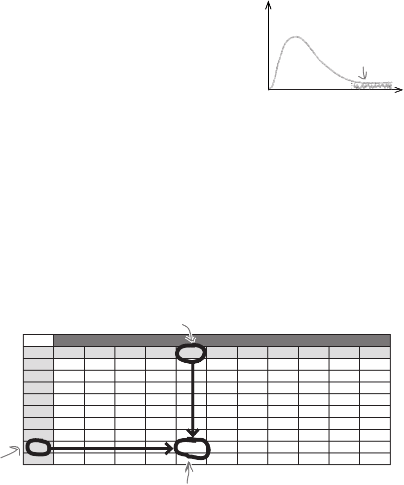
How to use χ

probability tables

To find the critical value, start off with the degrees of freedom, ν, and

the significance level, α. Use the first column to look up ν, and the

top row to look up α. The place where they intersect gives the value x,

where P(χ

(ν) ≥ x) = α. In other words, it gives you the critical value.

As an example, if you wanted to find the critical value for testing at the

5% level with 8 degrees of freedom, you’d find 8 in the first column,

0.05 in the top row, and read off a value of 15.51. In other words, if

our test statistic Χ

was greater than 15.51, it would be in the critical

region at the 5% level with 8 degrees of freedom.

Here’s the

row for

ν = 8.

Here’s the column for 0.05.

This is where 8 and 0.05 meet.

So how do we find the critical region for the χ

distribution? We can use

probability tables.

576 Chapter 14

Hypothesis testing with χ

Here are the broad steps that are involved in hypothesis testing with the χ

distribution.

Decide on the hypothesis you’re going to test,

and its alternative

Find the expected frequencies and the degrees

of freedom

Calculate the test statistic Χ

Determine the critical region for your decision

See whether the test statistic is within the

critical region

Make your decision

Look familiar? Most of these steps are exactly the same as for other

hypothesis tests. In other words, it’s exactly the same process as before.

So are χ

tests really just a special

kind of hypothesis test?

A: Yes, they are. You go through pretty

much all the steps you had to go through

before.

Do I always use the upper tail for

my test?

A: Yes, if you’re conducting a hypothesis

test, you always use the upper tail. This is

because the higher the value of your χ

test

statistic, the more your observed frequencies

differ from the expected frequencies.

I think I’ve heard the term degrees

of freedom before. Have I?

A: Yes, you have. Remember when we

looked at how we can use the t-distribution

to create confidence intervals? Well, the

t-distribution uses degrees of freedom, too.

I think I’ve seen degrees of freedom

referred to as df rather than ν. Is that

wrong?

A: Not at all. Different text books use

different conventions, and we’re using ν.

At the end of the day, they have the same

meaning.

I want to look for information about

the χ

distribution on the Internet. How do

I find it? Do I need to type in Greek?

A: You should be able to find any

information you need by searching for the

term “chi square.” The χ

distribution is also

written “chi-squared.”

These steps are

just like the ones

we had before

These steps are

different from the

ones you saw before

hypothesis testing steps

you are here 4 577

the χ

distribution

It’s your job to see whether there’s sufficient evidence at the 5% level to say that the slot

machines have been rigged. We’ll guide you through the steps.

1. What’s the null hypothesis you’re going to test? What’s the alternate hypothesis?

2. There are 4 degrees of freedom. What’s the region for the 5% level?

3. What’s the test statistic?

4. Is your test statistic inside or outside the critical region?

5. Will you accept or reject the null hypothesis?

Hint: You calculated this earlier.

578 Chapter 14

It’s your job to see whether there’s sufficient evidence at the 5% level to say that the slot

machines have been rigged. We’ll guide you through the steps.

1. What’s the null hypothesis you’re going to test? What’s the alternate hypothesis?

2. There are 4 degrees of freedom. What’s the region for the 5% level?

3. What’s the test statistic?

4. Is your test statistic inside or outside the critical region?

5. Will you accept or reject the null hypothesis?

: The slot machine winnings per game follow the described probability distribution.

: The slot machine winnings per game do not follow this probability distribution.

From probability tables, χ

(4) = 9.49. This means that the critical region is where X

> 9.49.

The test statistic is X

. You found this earlier; its value is 38.272.

The value of X

is 38.27, and as the critical region is X

> 9.49, this means that X

is inside the critical

region.

The value of X

is inside the critical region, so this means that we reject the null hypothesis. In other words,

there is sufficient evidence to reject the hypothesis that the slot machine winnings follow the described

probability distribution.

x -2 23 48 73 98

P(X = x) 0.977 0.008 0.008 0.006 0.001

exercise solution

you are here 4 579

the χ

distribution

Let’s summarize the steps you went through to discover this.

First of all, you took a set of observed frequencies for the slot machine and

calculated what you expected the frequencies to be, assuming they followed a

particular probability distribution. You then calculated the degrees of freedom

and calculated the test statistic Χ

, which gave you an indication of the total

discrepancy between the observed frequencies and those you expected.

After this, you used the χ

probability tables to find the critical region of the

distribution at the 5% level of significance. You checked this against your test

statistic and found that there was sufficient evidence to say that the slot machine

has been rigged to pay out more money.

Your test statistic fell in the critical region,

so you could reject the null hypothesis

This sort of hypothesis test is called a goodness of fit test. It tests whether

observed frequencies actually fit in with an assumed probability distribution.

You use this sort of test whenever you have a set of values that should fit a

distribution, and you want to test whether the data actually does.

You’ve solved the slot machine mystery

Thanks to your careful use of the χ

probability distribution, you’ve found out

that there’s sufficient evidence that the slot machine isn’t following the probability

distribution that the casino expects it to. Fat Dan is very grateful to you, as this

means you’ve come up with evidence that the slot machine has been rigged in

some way. He’s shut them down, so he doesn’t lose any more money.

(ν)

580 Chapter 14

Fat Dan thinks that the dice in the dice games are loaded. Take a look at the following

observed frequencies for one six-sided die, and test whether there’s enough evidence to

support the claim that the die isn’t fair at the 1% significance level. We’ll guide you through the

steps.

Here are the observed frequencies:

x Observed frequency Expected frequency

107

198

192

125

132

248

Value 1 2 3 4 5 6

Frequency

107 198 192 125 132 248

Step 1: Decide on the hypothesis you’re going to test, and its alternative.

Step 2: Find the expected frequencies and the degrees of freedom.

Start off by completing the expected frequencies for the die. You’ll need to take into account how many times the die is

thrown in total, and the probability of getting each value. X represents the value of one toss of the die.

Once you’ve found the expected frequencies, what are the number of degrees of freedom?

You find this the same way you

found the degrees of freedom for

the slot machines.

long exercise