Kallen A. Understanding Biostatistics

Подождите немного. Документ загружается.

Remarks on some estimation

methods

13.1 Introduction

We have a few loose ends to tie up before we conclude this book. They are all concerned

with estimation methods and model misspeciﬁcation and are mathematical in nature. The

mathematically less inclined reader may wish to skip these discussions, but is advised to have

at least a casual look, since we will address the analysis of some more complex data that may

be of general interest. We need to reiterate what was said in the preface – even if this chapter is

mathematical in nature, it is an overview, with less attention to details. The chapter is divided

into two main parts: the ﬁrst is a holistic discussion about estimating equations in general and

maximum likelihood theory in particular, and the second discusses how to analyze data with

repeated measurements within subjects.

We have often estimated parameters from an (estimating) equation U(θ) = 0, and used

the distributional properties of the stochastic variable U(θ) to obtain knowledge (e.g., con-

ﬁdence intervals) about the parameter θ. In the ﬁrst part of this chapter we will discuss this

approach in more generality. This will also help us to gain some understanding of why we

sometimes parameterize in θ, sometimes in its logarithm. We will link this to the well-known

maximum likelihood theory, which (essentially) is the special, but very important, case where

the estimating equation is the derivative of some function. This discussion will introduce a

special variance estimate, the robust variance, which is an alternative estimator of the vari-

ance also for likelihood estimators. The robust variance is less accurate than the one derived

from likelihood theory, but has the virtue of being less sensitive to model misspeciﬁcation,

since it is derived from the estimating equation alone. This gives us an opportunity to use the

wrong model and still draw the right conclusion. One illustration of this will be the analysis

of recurrent events in a heterogeneous population, a discussion that starts the second part of

this chapter.

Understanding Biostatistics, First Edition. Anders K¨all´en.

344 REMARKS ON SOME ESTIMATION METHODS

This second part continues the discussion on the subject-speciﬁc approach to dose

response, initiated in Section 10.6, except that this time we will not estimate the model

by reducing it to a population averaged model. Here we will take as our starting point the

likelihood for the problem. The problem with the likelihood approach for these non-linear,

though not for the linear, mixed-effects models is that their likelihood consists of multidi-

mensional integrals that are hard to compute accurately. Methods exist, but they are often too

computer-intensive at present for routine use, so we often need to use various approximations.

We will have a quick look at some of these approximations and demonstrate why we need

to understand how the estimation method works, in order to understand what we are actually

estimating – the population averaged or the subject-speciﬁc aspect of the problem.

13.2 Estimating equations and the robust variance estimate

The way we have carried out estimation in statistical models has mostly followed a certain

pattern. We start with a function U(x, θ) of the data x (both outcome variables and explanatory

variables) and an unknown parameter vector θ, such that the equation U(x, θ) = 0 deﬁnes

our estimate of θ as a function of x. Important examples of such functions U(x, θ) include

U(x, θ) = x

− θx

and U(x, θ) = x

− E

) used to estimate the odds ratio in

Section 5.3, the function



(x, θ)dF

(x) −

associated with the Wilcoxon test, and the

different functions discussed in Chapter 12, modeling survival data. Some of these will be

revisited below. The function U(x, θ), together with the sampling scheme, deﬁnes a stochastic

variable which depends on a parameter, which we denote by U(θ). The estimating equation

is then written as U(θ) = 0. As usual the point estimate of θ obtained from a particular set of

data is denoted θ

∗

, whereas the general solution of the equation (which is a function of the

data) is the estimator of θ, is a stochastic variable and is denoted by

θ.

The basic requirement on U(θ) is that it is unbiased, which in this case means that it has

mean zero:

(U(θ)) =



U(x, θ)dF

(x) = 0.

Here F

(x) is the CDF for the data set, a multidimensional CDF which we do not need to

be explicit about. It is important to note, and will be discussed further below, that it is the

equation that is unbiased; the estimator

θ need not be so. Usually the setup is such that we

have a stochastic variable X, representing a unit of data (data from one subject), together

with a function U(x, θ) such that E

(U(X, θ)) = 0, and we have at our disposal a set of n

independent observations x

of X from which θ should be estimated. This means that we

estimate θ from the average of the observed values of U(X, θ),



i=1

U(x

,θ) = 0.

(Note that when θ is a vector with s components, we need the estimating function to consist

of s independent components in order for this to be solvable.) This is useful, since it allows

us to appeal to large-sample theory when we wish to derive conﬁdence statements about θ.In

fact, we often appeal to the CLT to obtain that

U(θ) ∈ AsN

(0,V

(U(θ)).

ESTIMATING EQUATIONS AND THE ROBUST VARIANCE ESTIMATE 345

The key implication of this assumption is that

U(θ)

(U(θ))

−1

U(θ) ∈ Asχ

(s), (13.1)

which we can use to deﬁne the (approximative) conﬁdence function

C(θ) = χ

(U(θ)

(U(θ))

−1

U(θ))

for θ, from which we can subsequently deduce conﬁdence intervals and p-values. In order to

capitalize on this we need to know the variance or, at least, have an estimate of it. In some

cases where we only have an estimate of the variance to insert into the expression above, we

might wish to modify the distributional statement in equation (13.1) in order to obtain better

precision in the conﬁdence statements. If, for example, we analyze a linear model of Gaussian

variables we will have an F distribution after insertion of the sample variance as an estimate

of the true variance. In many other applications we instead appeal to large-sample theory and

keep the χ

(s) distribution, accepting that the results are approximate.

This discussion is the general version of approaches we have used for speciﬁc problems.

Now is the place to compare this with what is standard practice, which is to make one further

approximation in equation (13.1), in order to obtain an approximation to the variance of the

estimator

θ of θ. Recall from the deﬁnition of

θ that we have that U(

θ) = 0, which means that

when

θ is close to the true value θ, we have approximately that

0 = U(

θ) ≈ U(θ) + U



(θ)(

θ − θ).

This gives us a way (with the appropriate assumptions, which we ignore together with all

technical details) to ﬁnd an approximation to the distribution of

θ. For this we make one

further approximation and replace −U



(θ) with its expected value,

I(θ) =−E



(θ)),

which is called the information matrix (at least in the context of likelihood theory). This gives

us the approximation U(θ) ≈ I(θ)(

θ − θ), using which we can rewrite equation (13.1) as

(

θ − θ)

I(θ)

(U(θ))

−1

I(θ)(

θ − θ) ∈ Asχ

(s).

We therefore have that the variance of

θ is given, at least approximately, by the matrix

V (

θ) = I(θ)

−1

(U(θ))I(θ)

−t

We often compute this expression only at the point estimate θ

∗

of θ, and we also approximate

I(θ

∗

) with its observed value, the derivative −U



(θ

∗

). In order to compute V (

θ) we also need

an estimate of V

(U(θ

∗

)), which we obtain in the crudest of ways, by computing the average

−1



U(x

,θ

∗

)U(x

,θ

∗

)

. In all, this gives us an estimate of V (

θ) which is referred to as

the robust variance (another name often used is sandwich variance). It is robust in the sense

that if we have an estimating equation derived from some probability model, this estimate is

less sensitive to the validity of the modeling assumptions than the ordinary variance estimate

is. When we use this approximation to compute conﬁdence information, we refer to it as the

quadratic approximation of the conﬁdence function (around the estimate θ

∗

). The price paid

for using the robust variance estimate is that in general it is not a very efﬁcient estimator, and

we may need rather large samples in order to obtain reasonable accuracy.

346 REMARKS ON SOME ESTIMATION METHODS

We may note that even though we assume that there is an underlying probability model

which makes the stochastic variable U(θ) unbiased, this model is not really made explicit

anywhere when we use the robust variance. It is there in the background to assure that when

we estimate θ from the estimating equation, we are actually estimating a real parameter. We

do not use the probability model in any more explicit way.

By construction the stochastic variable U(θ) is unbiased, but that does not necessarily

mean that the estimate

θ is unbiased. It is not hugely biased, because

(

θ) ≈ θ + I(θ)

−1

(U(θ)) = θ,

an approximation which is better the larger the sample is. However, higher-order approxima-

tions may reveal some deviance to this, with resulting bias in small samples. This is further

discussed in Appendix 13.A.

For the rest of this chapter we will go through a few examples. All of these revisit dis-

cussions we have already had, but will provide some information about the relation between

different approximations. We also use these examples to highlight some further important

considerations, such as the importance of having the ‘right’ parameterization when we wish

to use the quadratic approximation. In the next section we will discuss the application of this

general theory to the special case of maximum likelihood estimation.

Example 13.1 In Example 12.4 we computed the two-sided conﬁdence function for the

log-rank test. The estimating function can be written as

U(θ) = N

(∞) −



∞

(t)

(t) + θY

(t)

(t),

and for its variance we have the estimate

V (θ) =



∞

(t)Y

(t)θ

(t) + θY

(t))

(t).

The conﬁdence function for θ is then obtained by applying the CDF for a χ

(1) distribution

to U(θ)

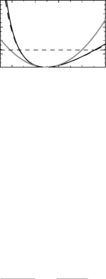
V (θ). This ratio, as a function of θ, is shown in Figure 13.1 as the solid black curve;

the corresponding 95% conﬁdence interval for θ is obtained as the intersection of this curve

with the 95th percentile for the χ

(1) distribution (shown as the dashed horizontal line).

There are two more curves in Figure 13.1. The gray curve is obtained from the quadratic

approximation based on θ. This requires that we compute the derivative of U(θ), which is

related to the variance estimate above through

V (θ) = θU



(θ). We therefore have that the

robust variance estimate is

I(θ)

−1

V (θ)

I(θ)

−1

= θ

V (θ)

−1

, with

I(θ) =−U



(θ), and the ratio

(θ − θ

∗

)

V (θ

∗

)/θ

∗

is what is shown as the gray curve in Figure 13.1. This is a quadratic

function, symmetric around the point estimate θ

∗

, and we see that it is in poor agreement with

the original function, deﬁning conﬁdence intervals that lie to the left of those derived from

the original function. (The reason why we plot the percentiles and not conﬁdence levels on

the y-axis is precisely to highlight the quadratic nature of this curve.)

However, if we write θ = e

and consider the expressions above as functions of β

instead, we have that

V (β) = U



(β). This does not change the black conﬁdence curve in any

way, because that approach is independent of how we parameterize. However, the quadratic

approximation depends on what parameterization we use: the quadratic conﬁdence curve for

β is (β − β

∗

)

V (β

∗

). Plotted versus β, this would provide a quadratic curve; in Figure 13.1

ESTIMATING EQUATIONS AND THE ROBUST VARIANCE ESTIMATE 347

54321

Hazard ratio

(1)-perc

entile

Figure 13.1 Conﬁdence information about the proportional hazards parameter from the

log-rank test, using three different approximations. For an explanation of the different curves,

see Example 13.1.

it is plotted versus θ = e

instead as the dashed curve. We see that although it differs

somewhat from the original curve, it is a good approximation to it in any region of interest

(which is deﬁned by the 95th percentile). The lesson is clear: when using the quadratic

approximation, it is important to choose the right parameterization. This, in turn, is related to

the choice of parameter scale in which the distribution of the estimator is best described by a

Gaussian distribution.

In the next example we revisit the problem of estimating conﬁdence intervals for per-

centiles of a distribution (previously discussed in Section 6.5).

Example 13.2 Let F

(x) be the e-CDF for a continuous variable, based on a sample of size

n. We wish to estimate the percentile θ = x

of the corresponding population CDF F (x). The

estimating equation for this is

U(θ) = F

(θ) − p = 0,

and we know that its variance is given by V (U(θ)) = V (F

(θ)) = F

(θ)

τ(θ), where

τ(θ) = F (θ)/nF

(θ) if there is no censoring; in the presence of censored data we estimate it

using the Greenwood estimator σ

of equation (11.7). The conﬁdence functions in the com-

plete and censored data cases are therefore χ

(x) applied to

n(F

(θ) − p)

p(1 − p)

and

(θ) − p)

(1 − p)

respectively. This is the approach that was explored in Chapter 6.

To investigate the corresponding quadratic approximation we need to compute the deriva-

tive of U(θ). For this purpose we redeﬁne the e-CDF F

(x) as its piecewise linear version

instead of the staircase version. We then have that U



(θ) = F



(θ), which is deﬁned at all points

θ except for the actual observations in the sample. This also implies that the information ma-

trix is I(θ) =−F



(θ), and it follows that

θ has the asymptotic variance F



(θ)

−2

V (F

(θ)). For

348 REMARKS ON SOME ESTIMATION METHODS

complete data this means that the asymptotic distribution for

θ is given by



θ,

p(1 − p)



(θ)



with a minor modiﬁcation for censored data.

We can also consider the problem of how to simultaneously estimate two percentiles

θ = (x

), where p<q. For this we deﬁne the two-dimensional estimating function

U(θ) = (F

(θ

) − p, F

(θ

) − q),

which is such that E(U



(θ)) is the diagonal matrix with entries F



(θ

) and F



(θ

). When

x<y, the covariance between F

(x) and F

(y)isgivenbyF

(x)F

(y)τ(x), from which

we can deduce what the variance matrix for θ looks like, how we should estimate it, and

how to obtain a two-dimensional conﬁdence function for θ. In particular, we ﬁnd that

the asymptotic correlation between ˆx

and ˆx

is τ(x

)/τ(x

), which for complete data re-

duces to

√

p(1 − q)/

√

q(1 − p). This addresses the problem discussed in Box 7.8 in a more

direct way.

In the next example we revisit the Mantel–Haenszel estimator of the odds ratio from an

estimating equation perspective.

Example 13.3 Consider a single 2 × 2 table, for which the conditional distribution of the

upper left element x

given the margins is the (non-central) hypergeometric distribution with

the odds ratio parameter θ. The estimating equation is

U(θ) = x

− θx

= 0,

the solution of which is the empirical odds ratio. Its variance is given by

(U(θ)) =

((x

+ θx

)(x

+ x

+ θ(x

+ x

))).

Here we can either compute this expression explicitly as a function of θ, which is the true

variance, or we can estimate it by inserting the observed values x

from the table cells and

get an estimated variance (still a function of θ). Furthermore,

I(θ) =−E



(θ)) =−E

) =−θ

−1

and if we denote the empirical odds ratio by θ

∗

, we see that the robust covariance estimator

for θ is given by θ

∗2

(θ

∗

), where

(θ) =

)

−2

+ θx

)(x

+ x

+ θ(x

+ x

)).

From this we also get the robust covariance estimate for the empirical log-odds ratio as V

(θ

∗

Another calculation shows that this is the variance for the logged odds ratio (see Section 4.5.1):

(θ

∗

) =

ESTIMATING EQUATIONS AND THE ROBUST VARIANCE ESTIMATE 349

(1)-percentile

5432

Odds ratio

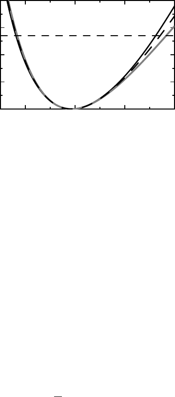
Figure 13.2 Deriving conﬁdence intervals for the odds ratio in a 2 × 2 table. The three

methods discussed in the text are illustrated.

We can graphically illustrate how this approximation works by comparing the

two functions

(θ) = U(θ)

(U(θ)) and Q

(θ) = (ln(θ) − ln(θ

∗

))

(θ

∗

We actually have two versions of Q

(θ): one in which we use the true variance and one in

which we use the estimated variance. These three functions are all illustrated in Figure 13.2 for

the ﬁrst Hodgkin’s lymphoma data set in Section 4.5.1. The solid black curve uses the function

(θ) with the true variance as a function of θ, while the gray curve is this function using

the estimate of this variance (still as a function of θ). The dashed curve, which is sandwiched

between these, is Q

(θ). The dashed horizontal line deﬁnes the intersection level for a 90%

conﬁdence interval, based on the χ

(1) distribution. We see that these functions are much in

agreement with each other at the lower conﬁdence limit, but disagree somewhat at the upper

limit. They agree with what we obtained in Figure 5.2 (dashed curves).

How to extend this to a general Mantel–Haenszel pooled odds ratio discussed in Section 5.5

is more or less immediate. The estimating function is the sum over strata,

U(θ) =



i=1

i11

i22

− θx

i12

i21

where n

is the total number of observations in table i. Applying the knowledge just

obtained for a single cell, we see that the variance in equation (5.3) is derived from the

robust variance for the estimating equation in the example, and is therefore what the quadratic

approximation for the log-odds ratio is based on.

This step from a single 2 × 2 table to a series of tables, that is, the introduction of a

stratiﬁed test, can be done in much larger generality. In fact, suppose we have a series of data

sets, each deﬁning an estimating equation U

(θ) = 0. We can then deﬁne a stratiﬁed test by

deﬁning the pooled estimating equation

U(θ) =



(θ) = 0

350 REMARKS ON SOME ESTIMATION METHODS

for some speciﬁed weights. In this way we can introduce both the stratiﬁed log-rank test

discussed in Section 12.7 and a stratiﬁed Wilcoxon test. In the latter case one usually takes

weights similar to those in the Mantel–Haenszel pooled odds ratio estimate.

Example 13.4 At this point we take a second look at the two quadratic forms discussed

in Section 5.5, which we called the Mantel–Haenszel and Breslow–Day quadratic forms.

If we have a series of N 2 × 2 tables with elements a

, the estimating equation

for the odds ratio for a single table is U

(θ) = a

− E

) = 0, where the expectation

is computed assuming a hypergeometric distribution. The pooled estimator function is

therefore U(θ) =



(θ), and a two-sided conﬁdence function can be obtained by

considering U(θ)

/V(U(θ)), which is the Mantel–Haenszel quadratic form. We derive the

conﬁdence function for θ by using the fact that this quadratic form has approximately a

(1) distribution.

The Breslow–Day quadratic form is the weighted least squares expression for θ. This is a

case where the parameter to be estimated also appears in the variance, and we therefore may

wisht to estimate the parameter using the GLS estimate. This produces precisely the same

estimating equation as above, so the two quadratic forms Q

(θ) and Q

(θ) deﬁne the

same test.

We could alternatively argue that Q

(θ) ∈ χ

(N) and derive a conﬁdence function from

this. However, similar to the discussion in Section 8.8, this contains two parts: the ﬁrst ad-

dresses whether it is reasonable that there is a common θ, and the second what we know about

such a θ. It takes more (individual strata cells need to be large; for Q

(θ) we only need to

have either large individual strata cells or many strata, or a combination) to get accuracy when

obtaining conﬁdence intervals for θ, and it is therefore not recommended. Instead we use it

for the other question: given the GLS estimate θ

∗

of θ, is this a reasonable summary of the

different tables? For this we compare Q

(θ

∗

)totheχ

(N − 1) distribution.

Our ﬁnal example in this section refers to the regression analysis in the Cox proportional

hazards model.

Example 13.5 The Cox proportional hazards model solves the equation

U(β) =



i=1



∞

− ¯z(t, β))dN

(t) = 0,

where

¯z(t, β) = ∂

ln S

(t, β),S

(t, β) =



i=1

(t)e

If we introduce our standard martingales ξ

(t) = N

(t) −



(s)e

d(s), the requirement

that the estimating equation is an unbiased estimator of β means that we can write

U(β) =



i=1



∞

− ¯z(t, β))dξ

(t).

MAXIMUM LIKELIHOOD THEORY 351

Its variance V

(U(β)) is given by

(U(β)

) = E





∞

(z − ¯z(t, β))

Y(t)e

zβ

d(t)



We also have that



(β) =−



i=1



∞

∂

ββ

ln S

(t, β)dN

(t),

and, under the assumption that the ξ

(t) are martingales, we see that the information matrix

I(β) is the same as E

(U(β)

). An alternative estimate of V

(U(β)) is



i=1





∞

(t) − ¯z(t, β))d

(t)



For the estimate

(t) we use the all-sample estimate of (t), which will be a function of β.

If we compute this at the point estimate β

∗

and multiply by the inverse of U



(β

∗

), we obtain

the robust estimator for the Cox model estimating equation.

This last example provides us with a way to analyze time-to-event data using the Cox

model also in situations where its model assumptions are not fulﬁlled, provided we use the

robust variance estimate, and have a sufﬁciently large sample. In Section 13.4 we will apply

this to the situation with recurrent events, where the assumption of independence of all events

cannot be assumed to hold.

13.3 From maximum likelihood theory to generalized

estimating equations

Our approach to parameter estimation has mostly been to deﬁne an equation that should hold

true for the correct parameter value. Usually in statistics parameter estimation starts with

likelihood theory, a methodology which we have also referred to occasionally. Here is the

place to see how this theory relates to that of estimating equations.

When we design an experiment we should (in principle) also have a probability model

for the outcome. The outcome is a sample, x = (x

,...,x

), and the probability model

is a (multidimensional) CDF F

(x) for the data. The likelihood theory asks the following

question: for which choice of θ is what we see most likely? This means that we introduce the

likelihood function

L(θ) = dF

(x),

computed at the point corresponding to the sample we obtained. For a continuous model this is

a density function, for a discrete model it is a probability function. Having already encountered

a number of examples of this, we proceed directly to the general theory. To obtain the maximal

value of the likelihood, which is also the maximum of ln L(θ), we solve the score equation,

U(θ) = (ln L)



(θ) = 0.

352 REMARKS ON SOME ESTIMATION METHODS

This implies that ∂

(x) = L



(θ) = U(θ)L(θ) = U(θ)dF

(x) (where ∂

denotes

differentiation with respect to θ), which in turn implies that ∂

(X) = E

(XU(θ)). The score

equation is the estimating equation of maximum likelihood theory, to which we can apply the

discussion we had in the previous section. However, it is an estimating equation with some spe-

cial properties. First we conﬁrm that it is unbiased, and therefore a valid estimating equation:

(U(θ)) =





(θ)

L(θ)

(x) = ∂



(x) = 0.

If we differentiate this equation we obtain from the differentiation formula above that



(θ)) + E

(U(θ)U(θ)

) = 0,

which means that in this case the information matrix equals the variance of the estimating

function, I(θ) = V

(U(θ)). This, in turn, implies that inference about θ is made from

U(θ)

I(θ)

−1

U(θ), a stochastic variable whose distribution is often assumed (appealing to

large-sample theory when our experiment is made up of a large number of independent

sub-experiments) to be at least approximately χ

(s), where s is the number of parameters.

The next problem is to obtain from this an expression for the variance of

θ. We addressed

this problem in the previous section, but we can do slightly more in this case, because U(θ)

is a derivative. We use a second-order Taylor expansion of ln L(θ) around the true value θ.

Inserting the maximum likelihood estimate into this gives the approximation

ln L(

θ) ≈ ln L(θ) + U(θ)

(

θ − θ) +

(

θ − θ)



(θ))(

θ − θ).

We also have that 0 = U(

θ) ≈ U(θ) + E



(θ))(

θ − θ), so

2(ln L(

θ) − ln L(θ)) ≈ (

θ − θ)

I(θ)(

θ − θ). (13.2)

If we can appeal to large-sample theory to deduce that U(θ) has an approximate Gaussian

distribution, the distribution on the right-hand side is approximately χ

(s), where s is the

number of components of θ. Applied to the right-hand side, it follows that

θ ∈ AsN

(θ, I(θ)

−1

In summary, we have three different expressions,

U(θ)

I(θ)

−1

U(θ), (

θ − θ)

I(θ)(

θ − θ), 2(ln L(

θ) − ln L(θ)),

all of which deﬁne (approximate) conﬁdence functions if we apply the CDF χ

(x)tothe

expression but replace the estimator

θ by the maximum likelihood estimate θ

∗

. Often we also

replace the matrix function I(θ) by the observed matrix −U



(θ

∗

) in the ﬁrst two expressions

here. The last expression deﬁnes a test which is referred to as the likelihood ratio test.

So far we have assumed that we are analyzing the correct model, but if we combine the

discussion here with that in the previous section, we can also use the score equation as an

estimating tool when the model is not correct, as long as we mitigate the misspeciﬁcation by

using the robust variance estimate instead of the model-derived one. This makes the analysis

less precise, compared to if the model had been correct, but there must be a price to pay for

using the wrong model. As an example, suppose that we want to do a classical ANOVA on