Kallen A. Understanding Biostatistics

Подождите немного. Документ загружается.

MAXIMUM LIKELIHOOD THEORY 353

Box 13.1 Proﬁle likelihood and restricted maximum likelihood

If we estimate parameters with the maximum likelihood method in the presence of

nuisance parameters, how do we eliminate these in a correct way from the analysis?

The general theory assumes we carry them with us all the way. One alternative is

proﬁling, which means that if θ = (θ

,θ

), where θ

represents nuisance parameters,

we deﬁne the proﬁle likelihood P(θ

) = L(θ

(θ

)), where

(θ

) is the maximum

likelihood estimate of θ

given that we know the value of θ

. This is not a true likelihood,

but sensible statistical analysis is often possible by imitating the likelihood ratio test

and deﬁning an approximate conﬁdence region for θ

from

{θ

; χ

(−2ln(P(θ

)/P(

))) ≤ 1 − α}.

In the particular case where we have data that are N(m, σ

)-distributed, and we want

to do inference about m by proﬁling σ

out, a short computation shows that

P(m)

P(¯x)



1 +

n − 1



−n/2

,t=

√

n(¯x − m)/s,

so the relative proﬁled likelihood is proportional to the density function for the

t(n − 1) distribution.

If we instead regard σ as the parameter of interest and m as the nuisance parameter,

the approximation is less satisfactory (though not bad). In that case there is an alternative

method, called restricted maximum likelihood, which also works for more complicated

Gaussian models, including the linear mixed effects model, when one wants to obtain

unbiased inference about variance information from likelihood theory. The basic idea

is that the residuals r

= x

− ¯x, follow a multivariate Gaussian distribution with mean

zero and a variance matrix which is given by σ

(I − e

e), where e = (1, 1,...,1).

This means that the maximum likelihood estimate f

−1



of σ

is unbiased, where

f = n − 1 is the dimension of the space orthogonal to the line deﬁned by e, and we end

up with the standard sample variance s

as the estimate for σ

. The general Gaussian

case with a linear model for the mean and potentially a complicated covariance structure

can be handled in the same way.

data that look far from Gaussian in distribution. We then use the estimating equation U(θ) = 0

derived from the likelihood theory for the ANOVA model, but use the robust variance estimate

when we compute conﬁdence intervals and p-values.

Example 13.6 We wish to illustrate this by applying the standard ANOVA without the

interaction term to the data discussed in Example 9.2. This means that we suggest a model

p = θ

+ θ

instead of the corresponding model for the log-odds. The outcome data, a dichotomous vari-

able, are obviously not Gaussian in distribution. As said, we analyze this binary data with

a standard ANOVA, but use the robust variance for conﬁdence statements. (Details on how

the robust variance estimator is computed in this case are given below.) Once this is done,

354 REMARKS ON SOME ESTIMATION METHODS

we transform the estimate of p, with its associated conﬁdence limits, into the log-odds by

means of the transformation p → p/(1 − p). The following table compares the result of this

analysis with that of the original logistic regression:

Logistic regression ANOVA

Parameter Estimate 95% CI Estimate 95% CI

Patients, Study 1 0.532 (0.264, 0.800) 0.528 (0.267, 0.809)

Patients, Study 2 0.147 (−0 .0761, 0.370) 0.149 (−0 .0715, 0.373)

Control, Study 1 −0.268 (−0.529, −0.00638) −0 .265 (−0.527, −0.0114)

Control, Study 2

−0.653 (−0.805, −0.50) −0.653 (−0.812, −0 .502)

We see that the actual conclusion from the study is not sensitive to how we arrived at it. The

methods differ, but they still provide very similar results.

The result in this example is very important, because it is the starting point for the method

of generalized estimating equations (GEEs). This methodology is used in cases where we

want to model clustered data, where clusters are independent but observations within clusters

are not. A typical situation is when we have serial measurements of an outcome variable,

so-called longitudinal data, in which the sets of data taken for individual patients are the

clusters. There are different ways to approach the analysis of such data, one of which is based

on specifying models for the data in the clusters, a kind of approach which we can think of as

subject-speciﬁc and which we will discuss further in Section 13.5. With the GEE technique

we instead take a population averaged approach in which we try to model the behavior of the

population mean values as a function of time and other covariates. The simplest application of

the GEE philosophy is to ignore all dependence between observations within individuals and

estimate the model using a simple GLM, except that when we compute conﬁdence statements,

we use the robust variance estimate instead of the model-based one. Often the GEE technique

is further reﬁned by introducing some tentative, but simple, form of dependence between

observations within clusters and modifying the estimating equation by weighting with the

appropriate variance matrix, much as we did in Section 10.6. Also when we use this empirical

model we still accept that this is not the correct model, and use the robust covariance estimate

for variance estimation. Our hope is that if we can capture some of the variability this way,

we may get a more efﬁcient robust covariance estimator.

In Example 13.6 we used the robust variance estimator for a GLS estimate, as deﬁned

by equation (9.1). We conclude this section by providing some computational details that are

applicable to models based on distributions from the exponential family.

Example 13.7 Consider the regression model of Y on X for which E

(Y|X = x) = f (θ, x),

and introduce the stochastic variable

U(θ) = f



(θ, X)

(Y − f (θ, X))/σ

(θ, X).

Since E

(U(θ)|X = x) = 0 for all x, we have that the variance of U(θ) is the expected value

of the conditional variances V

(U(θ)|X = x), given by



(θ, x)

(Y|X = x)f



(θ, x)/σ

(θ, x).

Since σ

(θ, x) = V

(Y|X = x), we have V

(U(θ)|X = x) = f



(θ, x)



(θ, x)/σ

(θ, x).

THE ANALYSIS OF RECURRENT EVENTS 355

Next we consider the information matrix. The derivative of U(θ) when X = x consists of

−f



(θ, x)



(θ, x)/σ

(θ, x) plus a term involving Y − f (θ, x) for which the mean is zero. Its

expected value (conditional on X = x) is therefore the same as above, and under the modeling

assumption the information matrix is the same as the variance of the estimator. Finally, the

model-free estimate of the variance of U(θ)is



i=1

U(x

,θ)U(x

,θ)



i=1

σ(θ, x

)

−4



(θ, x

)



(θ, x

)(y

− f (θ, x

))

Combining this with the information matrix above gives the robust variance for GLMs.

13.4 The analysis of recurrent events

To further illustrate that we can analyze a misspeciﬁed model for our data and still make an

acceptable inference by using the robust variance estimator, we now study the problem with

recurrent events that was introduced in Section 11.6. In that discussion we did not illustrate

the analysis with any examples, because we wanted the robust variance introduced ﬁrst. We

now have it, so we will remedy that omission in this section. We noted in Section 11.6 that we

cannot readily apply methods developed for single events in individuals to data consisting of

recurrent events within individuals, because it requires a crucial assumption: all events must

be independent, which would not be consistent with an expected patient heterogeneity in, for

example, disease severity. As noted then, the simplest way to handle this problem is to reduce

the data to the total number of events for each individual, ignoring when in time individual

events occur. Instead we assume that there is, for each individual, a mean intensity over

the period, deﬁned by the expected number of events, divided by the observation time. If we

assume that all individuals have the same constant hazard, with events occurring independently

of each other, we could analyze these count data as a Poisson regression problem, adjusting

for observation time. However, neither the assumption of homogeneity between patients, nor

the within-patient independence of events, is likely to hold. This suggests the possibility of

overdispersion, as illustrated in the next example.

Example 13.8 In a one-year study the investigators wanted to assess the effect on the

occurrence of asthma exacerbations when a long-acting brochodilator drug (LABA) was

added to an inhaled corticosteroid (ICS). The particular study had four treatment arms deﬁned

by two doses of ICS, separated by a factor of 4, each of which was studied with and without

concomitant administration of the LABA. We will analyze this in two steps, as discussed

in Chapter 9, and ﬁrst analyze the number of exacerbations using a Poisson regression

model approach.

In this step we estimate the group means of the exacerbation rates, adjusting for possible

predictive factors for exacerbations. One set of predictors are related to the fact that patients

with more severe asthma are expected to have more exacerbations. Both the FEV

as percent-

age of predicted normal

and the log of the ICS dose at enrollment were considered to be such

variables. Other covariates included were body mass index and sex, together with the basic

indicator variables for the four treatment groups. With these variables in a Poisson regression

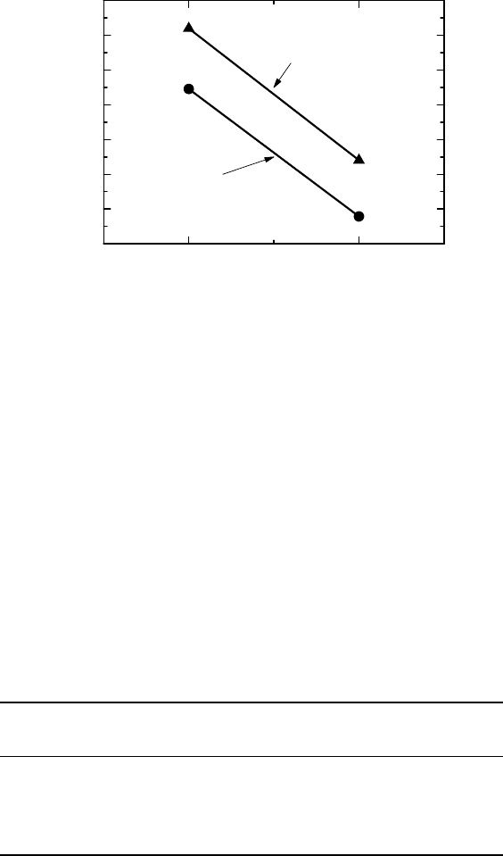
model, the output provides us with the adjusted exacerbations rates shown in Figure 13.3.

This is a prediction of what FEV

should have been for a healthy individual of the same height, age and sex.

356 REMARKS ON SOME ESTIMATION METHODS

0.2

0.3

0.4

0.5

0.6

0.7

0.8

0.9

Exacerbation rate

highlow

Dose of ICS

With LABA

Without LABA

Figure 13.3 Estimated exacerbation rates from a Poisson regression model.

These rates are adjusted to a common value for each of the covariates, which means that they

describe a situation where we have equal numbers of males and females in the groups, and

the other covariates are set to their overall study mean.

A Poisson model implies that all events, within and between subjects, are independent.

This is most likely a model misspeciﬁcation, because heterogeneity is expected to increase the

variance relative to what the standard Poisson model gives. There are two immediate remedies

for this, based on the Poisson model:

1. We can introduce an overdispersion factor (see Section 9.7) in the Poisson model.

2. We can use the robust variance estimate.

The table below shows how these three models compare in terms of the standard error for

the log-rates. (Note that the model analyzes log-rates, whereas we have plotted the rates in

Figure 13.3). The ratio between the standard error for the model with and without overdisper-

sion is constant, with the overdispersion parameter estimated to be 1.8. Going forward, we

will use the method with the robust variance.

Standard error

Treatment log(rate) Poisson Overdispersion Robust

ICS low −0.198 0.084 0.149 0.121

ICS low+LABA −0.437 0.093 0.164 0.151

ICS high −0.820 0.109 0.192 0.139

ICS high+LABA −1.278 0.134 0.237 0.169

This is the ﬁrst step, and is about ﬁnding comparable mean group estimates. In the second step

we want to compare these means in different ways, for which we may proceed in different

ways, depending on what the question is. The standard way to express the results is in terms

of hazard ratios: how much has the addition of a LABA, or an increase in the ICS dose,

decreased the hazard? Such information is obtained directly from the Poisson regression by

THE ANALYSIS OF RECURRENT EVENTS 357

forming linear combinations of the model parameters, followed by an exponentiation. We will

present the result in the next example.

An alternative second-step question may be this: how much should the ICS dose be

increased, in order to achieve the same effect on the exacerbation rate as is obtained by adding

the LABA? The two lines in Figure 13.3 represent two dose–response curves, one with and

one without the LABA, and since they look parallel it is a natural question to ask what the

relative (ICS) dose potency is. This means ﬁtting two parallel lines to the vector of estimated

rates λ

∗

. We therefore need to ﬁnd parameters θ = (θ

,θ

) such that the function

(θ

,θ

+ θ

ln(θ

),θ

+ θ

ln(4),θ

+ θ

ln(4θ

)),

where θ

represents the relative dose potency, has an optimal ﬁt to λ

∗

. This analysis should be

performed weighted by the covariance matrix for λ

∗

, for which we do not have an estimate.

The original Poisson analysis is done on the log-rates, so what we have is an estimate 

∗

the covariance matrix for these. We therefore need to transform our analysis to the log scale.

This means that we solve the GLS equation



(θ)



∗

−1

(ln(λ

∗

) − f (θ)) = 0,

where f (θ) is the logarithm of the function above. The corresponding parameter estimates

are θ

= 0.82,θ

=−0.27, and θ

= 1.85, and we see that we estimate that the effect on

the exacerbation rate of adding the LABA is equivalent to increasing the ICS dose by a

factor of 1.85.

The analysis in this example is a population averaged approach; claims are related to overall

group behavior and it uses the robust variance estimate (or an overdispersion parameter) to

mitigate a misspeciﬁed statistical model. Overdispersion can arise in a number of ways which

cannot be distinguished when we only have the aggregate count available. One likely cause

is heterogeneity in disease severity, which we may model by the frailty model. This model

assumes that rates are stable within patients during the whole study period, but may differ

between them. If we assume a gamma distribution for the frailties, we replace the Poisson

distribution with the negative binomial distribution, as was shown in Section 11.6.

Example 13.9 We now apply the negative binomial distribution to the data instead, using

the same linear model for the mean as in the last example. The following table shows the

group comparisons of primary interest, which are compared for the two models – the Poisson

model with the robust variance, which is a population averaged approach, and the negative

binomial model, which is a subject-speciﬁc approach.

Variable Parameter Estimate 95% CI p-value

Poisson ICS low±LABA 0.787 (0.578, 1.07) 0.20

(robust ICS high vs low 0.537 (0.397, 0.727) 0.00074

variance) ICS high±LABA 0.632 (0.444, 0.901) 0.033

Negative ICS low±LABA 0.761 (0.544, 1.07) 0.18

binomial ICS high vs low 0.481 (0.341, 0.678) 0.00045

ICS high±LABA 0.592 (0.404, 0.868) 0.024

358 REMARKS ON SOME ESTIMATION METHODS

We see that the ratios are in reasonable agreement, and also that the precision in these estimates

is similar for the two models.

So far we have not used all the available data, but only the reduced data set consisting

of the total number of events experienced for each patient. One way to analyze the complete

data is to use the estimating equation we would have used if all events were independent, and

then use the robust variance estimate for inference. Alternatively, we can model the data with

a frailty model, assuming that events within subject occur independently (given the degree

of frailty).

Example 13.10 In order to analyze all exacerbation data (including precise timings), we

next carry out a Cox regression, but instead of the standard model variance, we use the robust

variance when we make inference about parameters. This is the upper half of the table below,

which should be compared to the corresponding part of the table in Example 13.9. The main

difference is that not only is the precision increased, but also there is a slight numerical increase

in effects.

Variable Parameter Estimate 95% CI p-value

Cox model ICS low±LABA 0.825 (0.676, 1.01) 0.11

(robust ICS high vs low 0.617 (0.495, 0.767) 0.00028

variance) ICS high±LABA 0.658 (0.501, 0.865) 0.012

Frailty ICS low±LABA 0.806 (0.660, 0.985) 0.077

model ICS high vs low 0.615 (0.494, 0.766) 0.00026

ICS high±LABA 0.654 (0.496, 0.863) 0.012

The lower half of this table shows a random effects analysis of all data, which is analogous to

the previous use of the negative binomial distribution. It is an extension of the Cox regression

model to accommodate gamma frailties, assuming independence between events within a

subject, but allowing for subject-speciﬁc exacerbation rates. Such a model is called a shared

frailty model, and will be brieﬂy discussed in the next section. If we compare the result of

this analysis with the corresponding analysis of total count only, we see numerically larger

effects, together with increased precision. If we compare the two models in the table above,

we see that they are in reasonable agreement, in terms of both estimates and precision.

We have so far not discussed how to describe the complete set of exacerbation data in

order to ﬁnd out if there is some pattern to when exacerbations occur. One way to do this

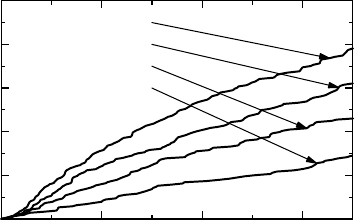
is to describe the data on a mean level and compute the mean cumulative function (MCF),

which is simply the average number of events that have occurred up to a given time point.

For the Poisson model, its cumulative intensity (t) is also its mean, and therefore the MCF.

In a heterogeneous world, where different individuals experience events, independent within

individuals, according to cumulative intensities (t, θ), with θs distributed as P(θ)inthe

population, the MCF becomes

m(t) =



(t, θ)dP(θ).

THE ANALYSIS OF RECURRENT EVENTS 359

0.2

0.4

0.6

0.8

MCF m (t)

3002001000

Time t (days)

ICS low

ICS low+LABA

ICS high

ICS high+LABA

Figure 13.4 The estimated mean cumulative functions describing exacerbations for

each treatment.

When the θs represent (proportional) frailties (i.e., when (t, θ) = θ(t)) this means that the

MCF is actually proportional to (t), with the proportionality constant being the average

value of the frailty distribution. In light of this, it is useful to plot the observed MCFs for

different groups, in order to see if they appear to have such a simple relationship to each other.

The estimation of the MCF is done by a Nelson–Aalen type of estimator. We write m(t)



dm(s) and estimate dm(t) by the number of observed events at time t, divided by the

number of individuals at risk at that time. The estimated MCFs for the data above are shown

in Figure 13.4, where we see that it is reasonable to consider these curves to be proportional

to some underlying mean function. There is therefore some support for the notion that the

frailty model is a reasonable explanation for much of the overdispersion.

We can also use the MCF and derive nonparametric tests similar to those in Chapter 12,

using the MCF instead of the cumulative hazard function in the derivation. The (minor) prob-

lem here is to account for the dependence structure in the variance estimate. We will not

pursue this; instead we will note a connection between this discussion and the one on com-

peting risks. The MCF description corresponds to the Kaplan–Meier estimate in conventional

survival analysis in that we estimate effects in an environment free of competing risks. This

is probably relevant in our situation, since the censoring reasons mainly were planned ones

(termination of study), or because patients were withdrawn by other (hopefully independent)

reasons. However, in some other settings, for example if we look at recurrent tumors after a

primary treatment course, it may be highly relevant not to ignore one particular competing

risk, namely that of death. We want statements not in an environment free of death, but in

its presence. This leads us into the same discussion as we had in Section 11.4, where we

replaced the survival function with the cumulative incidence function. In this case we replace

the MCF (which reduces to the survival function when there is only one event per patient)

with something that reduces to the CIF when there is only one event per patient. If F (t)is

the CDF for the time-to-death variable and μ(t) the conditional mean number of events in the

subset of individuals still alive at time t, the new MCF is

m(t) =



(s−)dμ(s).

360 REMARKS ON SOME ESTIMATION METHODS

This function is estimated using the Kaplan–Meier estimate for survival and a Nelson–Aalen

type of estimator for dμ(t). From there on we can obtain new tests. The whole approach

is similar to the replacement of the conventional log-rank test with Gray’s test in a

competitive environment.

13.5 Deﬁning and estimating mixed effects models

The recurrence data of the previous section is an example of clustered data, which means

that the observations come in clusters, or groups, so that all data are not independent. The

cluster may be the data from a patient on whom we repeatedly measure an outcome variable,

such as on different doses of a particular drug. Alternatively, it may be measurements taken

at different time points, as is the case in a longitudinal study. It could also be an account of

all the exacerbations, with timings, a patient experiences during the period he is observed.

The general setup is that we have n clusters (say, patients), and for each of these we have a

varying number n

of observations y

of the outcome variable. Let y

= (y

,...,y

) denote

the whole vector of observations for patient i.

We have encountered data of this kind in two examples so far. The ﬁrst was the dose–

response discussion in Chapter 10, where we have, for each of 20 individuals, ﬁve different

observations at different dose levels. For each individual we had a dose–response function

of a speciﬁc form, but with a subject-speciﬁc parameter, the ED

. The other example is the

toxicological experiment in rats in Example 12.1. So far, when we have analyzed these data, we

have done so under the assumption that the survival times for the 150 rats are all independent.

However, the data come from 50 litters with three pups in each. Rats from the same litter

are more closely related genetically than rats from different litters, which means that there

could be some correlation between lifetimes for rats within litter. In other words, there might

be a litter-speciﬁc frailty, ignorance of which might affect our result. In situations like these,

the likelihood is built up as a product of likelihoods for individual clusters. (We assume that

clusters are independent.) We will now discuss what the likelihood for such clusters looks like

in a few situations. Once we have done that, we can apply the general maximum likelihood

theory to the estimation of whatever model parameters are part of the problem. The model that

is applicable to the dose–response case was deﬁned in Example 10.6.1, and we start with it.

Example 13.11 In the notation above, the model that was speciﬁed in Example 10.6.1 is

that for each individual i, the n

= 5 observations y

∈ N(f (θ, D

),σ

) are independent, with

the function f (θ, D) = D/(e

+ D) describing the dose response for an individual. We also

assumed that θ ∈ N(μ, η

). Given that we know θ and σ

, the density of the distribution for

the vector y

is given by

|θ, σ

) = (2πσ

)

−n

−Q(y

,θ)/2σ

, where Q(y

,θ) =



j=1

− f (θ, D

))

The likelihood for a randomly sampled individual is obtained by taking the average of θ,

weighted according to the N(μ, η

) distribution:

(μ, η, σ) =



|θ, σ

)d



θ − μ



DEFINING AND ESTIMATING MIXED EFFECTS MODELS 361

A change of variable in this integral shows us that the total likelihood can be written as

L(μ, σ, η) = e

−n ln(σ)





−Q(y

,μ+

√

2ηξ)/2σ

−ξ

dξ,

up to a multiplicative constant. Here each integral is one-dimensional, so it is relatively

simple to compute it numerically to a reasonable precision using an appropriate integration

method. In order to estimate parameters, and derive conﬁdence information about these, we

use maximum likelihood theory. When we do so, we ﬁnd that the estimate of the mean of

is 0.79 with 95% conﬁdence interval (0.41, 1.50), which is compatible with the known

value of 1 (recall that these were simulated data). Moreover, we estimate the between-subject

variability (η) to be 1.42, and the within-subject variability (σ) to be 0.11, both of which are

in good agreement with the true numbers (

√

2 and 0.1, respectively). This is the method we

referred to in Section 10.6 as being the preferred method for the analysis of these data.

Example 13.12 We now construct the rat model in a similar way. For litter i we have three

intensity functions 

(t),j = 1, 2, 3, for the three pups. The assumption we make is that



(t) = ηz



(t), where 

(t) is a reference intensity common to all, z

is one if the rat is

a control and it equals θ if the rat is treated with the drug (θ is the hazard ratio, describing

the treatment effect), and η is a litter-speciﬁc frailty. Within litter we assume that lifetimes

for pups are independent so, if we knew the frailty of a particular litter to be η, the survival

function for that litter would be



−ηz



)

= e

−η





)

Since we do not know η, we average over it to get



∞

−η





)

dP(η) = L

⎛

⎝





)

⎞

⎠

where L(s) is the Laplace transform of the frailty distribution P(η). The corresponding prob-

ability density is obtained by differentiation, and repeating some of the calculations we did

earlier gives us the log-likelihood

L(θ, α) =



i=1

⎛

⎝

⎛

⎝



j=1

d

)

⎞

⎠

+ ln

⎛

⎝

(−1)

(δ

)

⎛

⎝



j=1



)

⎞

⎠

⎞

⎠

⎞

⎠

The parameter θ, which describes the treatment effect, is hidden in the z

, and α deﬁnes the

distribution P(η). A model of this kind is called a shared frailty model; in this case the frailty is

shared between the pups in a litter. If we have a parametric representation of 

(t), parameter

estimation is a classical maximum likelihood problem, but we can also carry out the analysis

in the more general case with an unspeciﬁed baseline hazard.

If we recall the close connection between the Poisson distribution and the Cox regression

model, it should come as no surprise that a popular choice is to take P(η) as a gamma

distribution with mean one. There are different numerical methods available for the analysis

of such a model which, when applied to our rat data, gives almost the same estimate for θ as

362 REMARKS ON SOME ESTIMATION METHODS

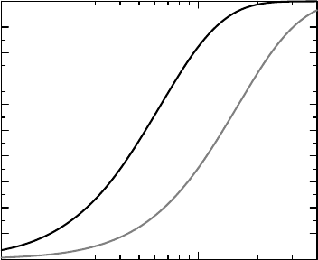
0.1

0.2

0.3

0.4

0.5

0.6

0.7

0.8

0.9

Proportion of rats

−1

Frailty parameter

Figure 13.5 The distributions of rat frailty in the two groups in the toxicological experiment.

was obtained in the analysis when clusters were ignored, namely 2.5 with 95% conﬁdence

interval (1.3, 4.7). The variance of the heterogeneity distribution is estimated to be 0.47.

To illustrate what this model implies, look at Figure 13.5 which shows the frailty distribu-

tions for each group. We see how the control animals have a frailty distribution that lies to the

left of that of the drug-treated ones. The drug effect is, according to the model, a multiplicative

constant, so on the log scale we should obtain two parallel (horizontally shifted) CDFs.

As already mentioned, another example of a shared frailty model is the recurrent exac-

erbation data discussed in the previous section, in which frailty for exacerbations is shared

within patients.

Both these examples illustrate mixed effects models of clustered data. Such models

can be constructed for a variety of data, where we start the modeling with a description of

what happens on the individual level by deﬁning a function of some parameters. Some of

these parameters may take different values in different individuals, and are then called

random parameters, whereas other parameters are the same for all individuals and referred

to as ﬁxed parameters. As before, the random parameters are described by a distribution,

which contains some unknown model parameters that we need to estimate. In addition

to this, the outcome variable will also have some associated variability that requires a

distribution describing it, again speciﬁed up to some unknown model parameters. When

there is more than one random parameter we usually need to account for the dependence

between them, which leads us to assume that the distribution for the random parameters

(or some simple transformation thereof, such as taking the logarithm) is a multidimensional

Gaussian distribution, because this is more or less the only model that can easily describe

the correlation between parameters. But there is a problem. The likelihoods of the clusters so

deﬁned are multidimensional integrals which in most cases cannot be explicitly computed. We

therefore need to resort to numerical methods, and numerical methods for higher-dimensional

integrals are computer-intensive. This has led to the introduction of various approximations,

approximations that do not necessarily provide us with what we are led to believe from our

initial model description. These approximations will be the subject of the rest of this section.