Kelly J.J. Graduate Mathematical Physics, With MATHEMATICA Supplements
Подождите немного. Документ загружается.

66 2 Integration
becomes available. If one needs to evaluate an integral, like
x
2n
x
2
x, that is pre-
sented without a parameter, simply insert one to obtain
x
2n
Λx
2
x
(
(Λ
n
Π
Λ
2n 1!!
2
n
Λ
n
1
2
(2.3)
and then set Λ!1. It might surprise you how often this trick is helpful.
Notice that if a parameter appears in the limits of integration, one must also include
the variation of these limits using
(
(Λ
bΛ
aΛ
f x, Λ Λ
b
a
( f x, Λ
(Λ
x f b, Λ
(b
(Λ
f a, Λ
(a
(Λ
(2.4)
with the rhs evaluated for the appropriate Λ.
2.2.2 Convergence Factors
Sometimes when it is not obvious whether the integral of an oscillatory function over an
infinite range will converge to a definite value, application of a convergence factor may
help resolve the question. For example, it is not obvious, at least to this author, whether
0
Sinkxx converges. Consider instead
0
Λx
Sinkxx Im
0
Λx
kx
x
Im
1
Λk
k
Λ
2
k
2
(2.5)
which does converge for Λ > 0. The desired integral is then obtained from the limit Λ!0,
whereby
0
Sinkxx lim
Λ!0
0
Λx
Sinkxx
1
k
(2.6)
Admittedly, this result does appear somewhat arbitrary and some skepticism is justified.
However, if this integral were encountered in a physics problem, it probably would arise
from a limiting process anyway. Either a spatial or temporal variable should be limited
to a finite range or a damping mechanism should be present that ensures convergence.
One should then retreat a few steps in the derivation, identify the appropriate convergence
factor, and evaluate the integral before that convergence factor is lost from view.
2.3 Contour Integration
2.3.1 Residue Theorem
Suppose that f z is analytic throughout a domain D except for isolated singularities
(poles) and that a simple closed contour C within D encircles poles z
k
,k 1,N with
residues R
k
. By deforming the contour to encircle each pole, we obtain
C
f zz
N
k1
C
k
f zz (2.7)

2.3 Contour Integration 67
where eachC
k
is a small circle encompassing pole k. Near each z
k
we can employ a Laurent
expansion
f z
nm
k
a
n,k
z z
k
n
C
k
f zz
nm
k
a
n,k
C
k
z z
k
n
z (2.8)
to evaluate its contribution to the contour integral. Using the now familiar circular contour
integration with z z
k
Ρ
Θ
z Ρ
Θ
Θ, we obtain
C
k
z z
k
n
z Ρ
n1
2Π
0
n1Θ
Θ 2Π∆
n,1
C
k
f zz 2Πa
1,k
2ΠR
k
(2.9)
Therefore, we obtain the residue theorem:
Theorem 18. Residue theorem: If f z is analytic on and within a simple closed counter-
clockwise contour C, except for interior poles z
k
,k 1,N with residues R
k
, then
C
f zz 2Π
N
k1
R
k
This is an amazingly powerful theorem that can be used, with clever choices of contour,
to evaluate a wide variety of definite integrals which might be very difficult by means of
familiar antidifferentiation methods. The trick is to find a simple closed contour that con-
tains the desired integral on one portion of the path with easier integrals on the remainder
of the path (if any). The examples in following subsections will demonstrate that contour
integration using the residue theorem provides some of the most versatile methods for
evaluating definite integrals.
2.3.2 Definite Integrals of the Form
2Π
0
f sin Θ, cos Θ Θ
We assume that f sin Θ, cos Θ can be represented by a single-valued function of z
Θ
in
the relevant region of the complex plane. Often f is a rational function of sin Θ and cos Θ.
Then we use
z
Θ
Θ
z
z
, SinΘ
z z
1
2
, CosΘ
z z
1
2
(2.10)
such that
2Π
0
f SinΘ, CosΘΘ
f
z z
1
2
,
z z
1
2
z
z
2Π
residues within unit circle
(2.11)
where the contour is the unit circle about the origin. Special handling is needed if any of
the singularities of f are on the unit circle.
68 2 Integration
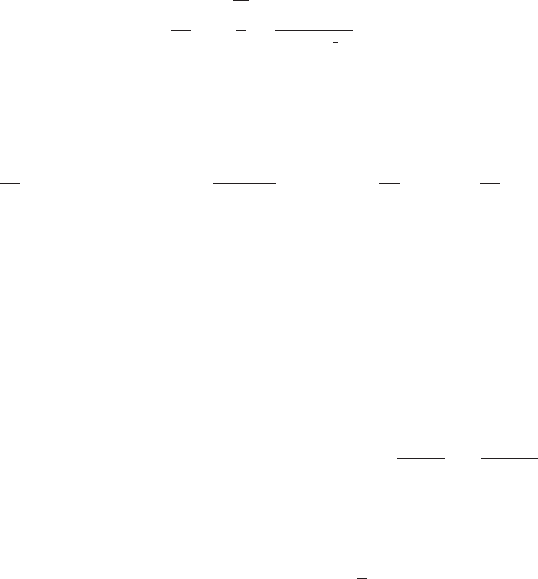
Figure 2.1. Poles in the integrand from Eq. (2.12). Left: Ima0. Right: Ima > 0.
2.3.2.1 Example: Ia
Π
0
a
a
2
SinΘ
2
Θ
Although this integral is not stated in the desired form, the integrand is even. Hence, by
direct application of the recipe above, we find
Ia
1
2
2Π
0
a
a
2
SinΘ
2
Θ4a
z
4a
2
z
2
z
2
1
2
z (2.12)
The denominator is a quadratic in z
2
, so that one obtains four poles at
denominator 4a
2
z
2
z
2
1
2
poles z/. Solvedenominator 0, z
a
1 a
2
,a
1 a
2
, a
1 a
2
,a
1 a
2
Evaluation of the residues
Map
Residue
z
denominator
, z, #
&, poles
1
8a
1 a
2
,
1
8a
1 a
2
,
1
8a
1 a
2
,
1
8a
1 a
2
is straightforward, even by hand. If a>0 the pair of poles at
a
1 a
2
is inside the
unit circle while the other pair is outside, while if a<0 the reverse is true. In either case
we have two equal contributions, such that
Ia
Π
1 a
2
(2.13)
Figure 2.1 illustrates the positions of the poles relative to the unit circle. The left figure
uses a real value for a, while the right figure uses a complex value. Although one typically
assumes that parameters in definite integrals are real, the method is more general and does
not require that assumption.
Alternatively, if we use a trigonometric identity to express the integrand as
a
a
2
SinΘ
2
/ . SinΘ
2
1 Cos2Θ
2
/ / Simpli fy
2a
1 2a
2
Cos2Θ
2.3 Contour Integration 69
we obtain a contour integral with a quadratic denominator
Ia
2Π
0
a
1 2a
2
CosΘ
Θ 2a
1
z
2
2
2a
2
1
z 1
z (2.14)
for which evaluation of the residues is easier by hand.
denominator z
2
2
2a
2
1
z 1
poles z/. Solvedenominator 0, z
1 2a
2
2a
1 a
2
,1 2a
2
2a
1 a
2
Map
Residue
1
denominator
, z, #
&, poles
1
4a
1 a
2
,
1
4a
1 a
2
Notice that there are only two poles in the transformed function because the angular vari-
able was replaced by Θ!Θ/ 2. Recognizing that for either sign of a just one of the poles is
within the unit circle, one obtains the same final result.
2.3.3 Definite Integrals of the Form
f xx
We assume that f z is analytic except for isolated singularities and vanishes faster than
z
1
for r !in either half-plane. With these conditions we can employ a semicircular
contour of radius R !closed in the appropriate half-plane to obtain
f xx
f zz 2Π
residues in half-plane (2.15)
To prove this result, suppose that f z is bounded in the upper half-plane such that
f
R
Θ
MR
Α
Π
0
f
R
Θ
Θ
MR
Α
ΠR (2.16)
where M is a positive real number. Then
Α > 1 lim
R!
Π
0
f
R
Θ
Θ
lim
R!
ΠMR
1Α
0
lim
R!
R
R
f xx 2Π
residues in half-plane
(2.17)
ensures that if f falls fast enough we need only evaluate the residues at isolated singulari-
ties of the analytic function f z in the appropriate half-plane. Therefore, we find
lim
R!
R
f
R
Θ
0 lim
R!
R
R
f xx 2Π
residues in half-plane (2.18)
using a great semicircle.
70 2 Integration
2.3.3.1 Example: Ia
1
1x
4
x
The integral
1
1 x
4
x
C
1
1 z
4
z (2.19)
can be evaluated using a semicircular contour in either half-plane. The integrand has poles
at z
k
ExpΠ
2k1
4
for k 1, 4 of which two are found in each half-plane. The residues
can be evaluated using
f z
1
qz
R
k
1
q
'
z
k
1
4z
3
k
1
4
3Π/ 4
k
1
4
2
k
(2.20)
Thus, we obtain
1
1 x
4
x
C
1
1 z
4
z 2Π
1
4
2
1
Π
2
(2.21)
2.3.4 Fourier Integrals
Consider a Fourier integral of the form
˜
f k
f x
kx
x (2.22)
where k is a positive real number. Integrals of this type can often be evaluated by extending
f to the complex plane and using a great semicircle in the upper half-plane, provided that
the contribution of the return path
I
R
kR
Π
0
f
R
Θ
ExpkRSinΘ CosΘ Θ (2.23)
vanishes in the limit R !. Suppose that M
R
is the maximum modulus of f on this arc,
such that
I
R
RM
R
Π
0
ExpkR SinΘ Θ (2.24)
Dividing this latter result into two equal contributions now gives
I
R
2RM
R
Π/ 2
0
ExpkR SinΘ Θ (2.25)
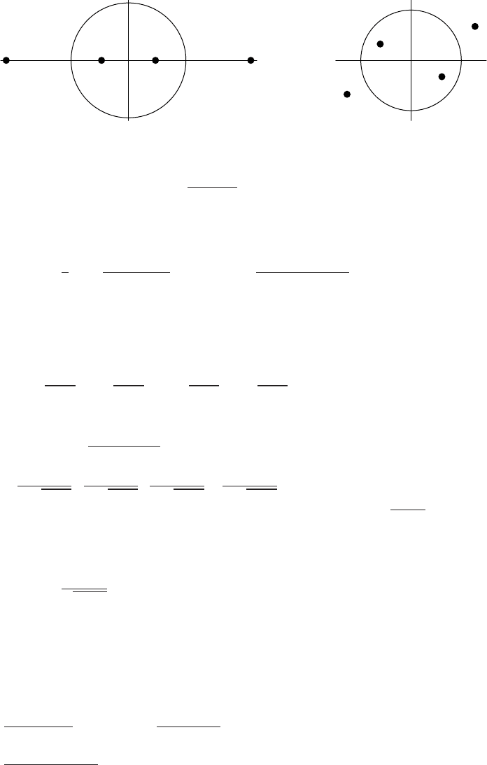
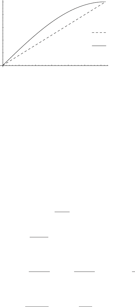
Figure 2.2 illustrates that SinΘ > 2Θ/Π on this interval. Thus, the integral on the great
semicircle is limited by
I
R
2RM
R
Π/ 2
0
Exp2kRΘ/ Π Θ (2.26)
or
I
R
ΠM
R
1
kR
k
(2.27)
2.3 Contour Integration 71
0.25 0.5 0.75 1 1.25 1.5
T
0.2
0.4
0.6
0.8
1
Sin#T '
2T sS
Figure 2.2.
This result is known as Jordan’s lemma. Therefore, if k>0 and if f z vanishes on an
infinite semicircle, such that
lim
R!
M
R
0
I
R
0 (2.28)
the contribution of the return path vanishes and we may evaluate the Fourier integral using
lim
R!
f
R
Θ
0
f x
kx
x 2Π
residues of integrand in half-plane
(2.29)
If k happens to be a negative real number, we close in the lower half-plane instead and
obtain the same result. Notice that this condition upon f is less restrictive than in the
previous section due to the presence of the exponential factor, which is damping in the
appropriate half-plane. However, convergence for k 0 requires lim
R!
R f R
Θ
0as
before.
2.3.4.1 Example:
0
Coskx
x
2
a
2
x
Consider the integral
˜
f k
0
Coskx
x
2
a
2
x (2.30)
where k and a are positive real numbers. Although this integral is not presented in the
desired form, it is simply half the real part of
˜gk
Expkx
x
2
a
2
x
Expkz
z
2
a
2
z
˜
f k
1
2
Re
˜gk
(2.31)
and may be evaluated using a great semicircle in the upper half-plane, wherein lies one
simple pole at z a. Therefore, we obtain
˜gk2Π
Expka
2a
˜
f k
Π
ka
2a
(2.32)
without further ado. The result is actually more general than this derivation – it applies
equally well for complex a provided only that Rea0 to ensure that the poles are not on

72 2 Integration
the real axis. Be alert to generalizations! Having expended some effort to obtain a result,
it is good practice to extend it to the most general conditions possible. Also notice that
one cannot use Cosaz/z
2
a
2
directly because Cosaz is not bounded on the great
semicircle – it diverges exponentially for large Imz in both upper and lower half-planes.
2.3.5 Custom Contours
Sometimes it is necessary to design a contour which exploits specific characteristics of
the integrand. For example, when previously evaluating the integral
0
Cosx
2
x we
employed an arc subtending Π/ 4 radians. Unfortunately, there are no general rules to guide
one toward the optimum contour for an arbitrary integrand; one must rely on intuition and
experience to minimize the amount of trial-and-error in choosing such contours. Below we
give just one more example of a custom contour.
Consider the integral
I
ax
x
1
x 0 <a<1 (2.33)
The integral on the real axis converges because the integrand is of order
ax
for x !
or Expa 1x for x !and decreases exponentially in either limit when 0 <a<1.
However, the function
f z
az
z
1
z
k
2k 1Π (2.34)
with simple poles on the imaginary axis at odd-integer multiples of Π does not satisfy the
conditions needed to employ a great semicircle. Fortunately, the contour integral
f zz lim
R!
R
R
f x, 0 x
2Π
0
f R, y y
R
R
f x, 2Π x
0
2Π
f R, y y
(2.35)
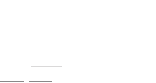
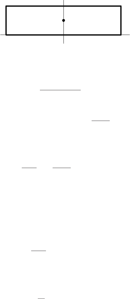
can be evaluated fairly easily using the rectangular strip, ( <x<, 0 y 2Π),
shown in Fig. 2.3. This contour encloses a single pole at z
0
Πwith residue
Πa
, such
that
f zz 2Π
Πa
(2.36)
The contributions from vertical segments
lim
R!
f R, y lim
R!
ExpaR y
ExpR y1
lim
R!
Expa 1R0 (2.37)
lim
R!
f R, y lim
R!
ExpaR y
ExpR y1
lim
R!
ExpaR0 (2.38)
2.4 Isolated Singularities on the Contour 73
x
y
Π
RR
2
Π
Figure 2.3. Rectangular contour used for Eq. (2.33).
vanish in the limit R !, while the horizontal segments are related by
f x, 2Π
Expax 2Π
Expx 2Π 1
Exp2Πa f x, 0 (2.39)
such that
f zz
1
2Πa
I I
Π
SinΠa
(2.40)
This result actually finds somewhat broader applicability because the contributions
from the vertical segments vanish provided only that 0 < Rea < 1. Therefore, we can
allow a to be complex and find
ax
x
1
x
Π
SinΠa
for 0 < Rea < 1 (2.41)
As always, be alert for possible generalizations.
2.4 Isolated Singularities on the Contour
2.4.1 Removable Singularity
Often one encounters isolated singularities on the integration path. For example, the inte-
gral
I
Sinx
x
x (2.42)
is important in Fourier analysis. The integrand has a removable singularity at the origin,
but that would not cause any difficulty if the integral remained in this form. However,
because Sinz is divergent as y !, we would prefer to evaluate
I Im
x
x
x (2.43)
by closing the contour in the upper half-plane. The penalty for this transformation is
that the singularity at the origin is no longer removable. Fortunately, that problem can
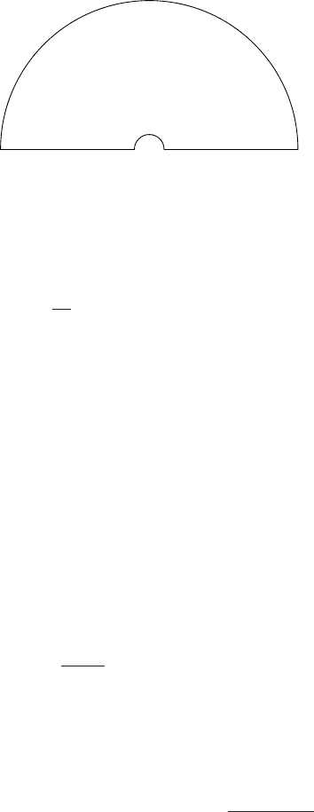
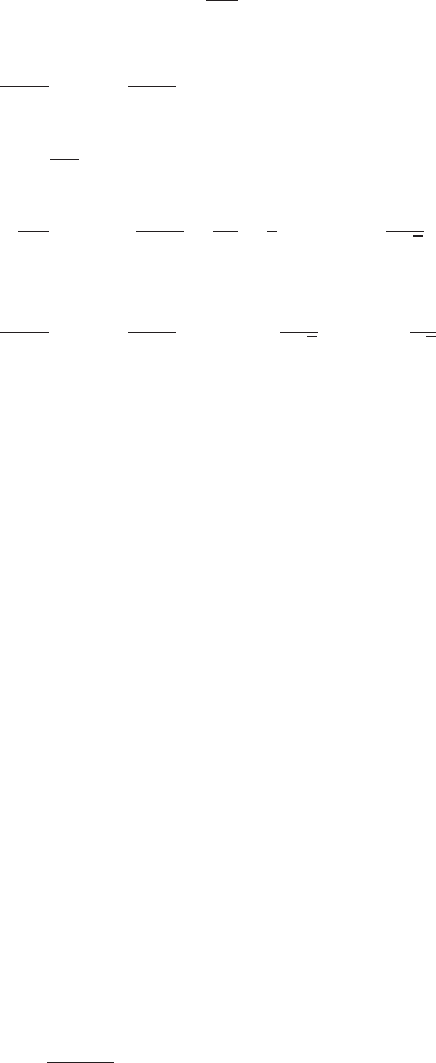
74 2 Integration
Figure 2.4. Great semicircle with small detour that excludes a removable singularity at the origin.
be avoided by also making a small semicircular detour around the origin as sketched in
Fig. 2.4. According to Cauchy’s theorem, the integral
z
z
z 0 (2.44)
vanishes on this contour because no singularities are enclosed. The contribution of the
great semicircle vanishes because the integrand satisfies the requirements of Jordan’s
lemma. The linear segments
lim
!0
f xx
f xx
(2.45)
converge to the desired integral in the limit ! 0 because the integrand is well-behaved
on the real axis. The contribution of the small semicircle of radius ! 0 is evaluated using
z z Θ
0
Π
f zz Θ lim
!0
0
Π
Exp
Θ
Θ Π (2.46)
Therefore, we find
Sinx
x
x Π (2.47)
Notice that the contribution of the semicircular detour is Π times the residue of the
integrand, half the value we would have obtained from the residue theorem for a complete
circle around the singularity. More generally, if f z is analytic at z
0
, the detour integral
z z
0
Θ
lim
!0
Θ$Θ
Θ
f
z
0
Θ
z z
0
z f
z
0
$Θ (2.48)
is proportional to the angle subtended. This result is easily proven by expanding f z
around z
0
. Also, notice that $Θ is positive for counterclockwise or negative for clockwise
detours.
2.4 Isolated Singularities on the Contour 75
2.4.2 Cauchy Principal Value
An improper integral whose integrand is singular at one of the endpoints of the integration
range is defined by one of the limits
b
a
f xx lim
!0
b
a
f xx or
b
a
f xx lim
!0
b
a
f xx (2.49)
However, if an isolated singularity lies within the range of integration then two limits are
needed
c
a
f xx lim
1
!0
b
1
a
f xx lim
2
!0
c
b
2
f xx (2.50)
and often there will be no unique value if the two limits are taken independently. For
example, applying this method to
1
1
x
x
lim
1
!0
1
1
x
x
lim
2
!0
1
2
x
x
lim
1
!0,
2
!0
log
1
2
(2.51)
does not provide an unambiguous result unless one decides to approach the singularity in
a symmetric manner, such that
1
2
. This particular value is designated the Cauchy
principal value of the integral and denoted by
, such that
c
a
f xx lim
!0
b
a
f xx
c
b
f xx
(2.52)
Hence, for the example above we find
1
1
x
x
0 (2.53)
If there are several isolated singularities on the contour, the Cauchy principal value treats
each symmetrically.
The Cauchy principal value is based upon antisymmetric behavior near a simple pole,
where we can write
f z
a
1
z z
0
gz (2.54)
with gz analytic near z
0
. As illustrated by Fig. 2.5, the two divergent contributions on
either side cancel, leaving behind the background contribution g. Of course, this cancella-
tion does not work for a double pole with symmetric divergence.
2.4.2.1 Example:
Coskx
a
2
x
2
x
Consider the integral
I
Coskx
a
2
x
2
x Re
Expkx
a
2
x
2
x
(2.55)
where a and k are positive real numbers. By replacing Cos with Exp we are able to close
the contour in the upper half-plane and use Jordan’s lemma to discard the contribution