Kusse B.R., Westwig E.A. Mathematical Physics: Applied Mathematics for Scientists and Engineers
Подождите немного. Документ загружается.

376
DIFFERENTIAL EQUATIONS
t
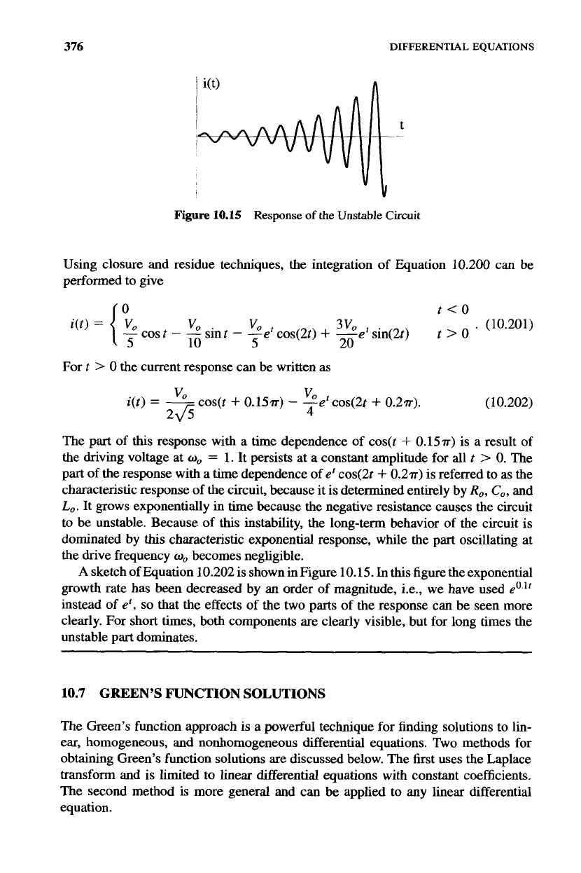
Figure
10.15
Response
of
the
Unstable
Circuit
Using closure and residue techniques, the integration of Equation 10.200 can be
performed to give
t<O
t
>
0
VU
vo
t
3vu
f
.
(10.201)
cost
-
-
sint
-
-e
cos(2t)
+
-e
sin(2t)
10 5
20
For
t
>
0
the current response can be written
as
(10.202)
The part of
this
response with a time dependence of cos(t
+
0.15~) is a result
of
the driving voltage at
w,
=
1. It persists at a constant amplitude for all t
>
0.
The
part of the response with
a
time dependence
of
er
cos(2t
+
0.2~)
is referred to as the
characteristic response of the circuit, because it is determined entirely by
R,,
Co,
and
Lo.
It grows exponentially
in
time because the negative resistance causes the circuit
to
be
unstable. Because of
this
instability, the long-term behavior of the circuit is
dominated by
this
characteristic exponential response, while the part oscillating at
the
drive
frequency
w,
becomes negligible.
A
sketch of Equation 10.202
is
shown
in
Figure 10.15.
In
this
figure the exponential
growth rate has been decreased by an order
of
magnitude, i.e., we have used
e0."
instead
of e',
so
that the effects of the two parts of the response can be seen more
clearly. For short times, both components are clearly visible, but for long times the
unstable part dominates.
"0
f
cos(t
+
0.1%)
-
-e
cos(2t
+
0.217).
4
i(t)
=
-
VU
2JJ
10.7
GREEN'S FUNCTION SOLUTIONS
The Green's function approach
is
a powerful technique for finding solutions to lin-
ear, homogeneous, and nonhomogeneous differential equations. Two methods for
obtaining Green's function solutions are discussed below. The first uses the Laplace
transform and is limited to linear differential equations with constant coefficients.
The second method is more general and can
be
applied to any linear differential
equation.
GREEN'S
FUNCTION
SOLUTIONS
377
10.7.1 Derivation
Using
the Laplace
Transform
Consider an ordinary, second-order, nonhomogeneous, linear differential equation
with constant coefficients
d2r(t)
+
Bod")
+
Cor(t)
=
d(t),
dt
A,
2
dt
(10.203)
where
r(t)
is the response to a known driving function
d(t).
The independent variable
f
is assumed to be time,
so
the concept of causality applies to the response. In other
words, the response cannot occur before the application of the driving term. Assume
the driving function
is
zero for
t
<
0,
and that it has a standard Laplace transform
D_(s).
The causal boundary conditions
are
r(0)
=
0
and
dr/dt\t=o
=
0.
The Laplace
transform of the differential equation becomes
+
Bog
+
C,)R_O
=
LW,
(10.204)
where
&s)
is the Laplace transform
of
the response. Equation 10.204 can be solved
for
&):
DO
A,s2
+
Bog
+
C,
'
=
which, in turn, can be inverted to give the response
(10.205)
(10.206)
So
far, this is nothing more than a recap of the Laplace transform approach to solving
differential equations, which we presented in the previous section. At this point,
however, we take a completely different tack.
Returning
to
the Laplace transform
of
the response, it can
be
looked at
as
the
product of two functions
=
QOG(d9
(10.207)
where
C(s)
=
1/(A,s2
+
Box
+
C,).
Consequently, from the product property of
Laplace transforms, the time domain response is the convolution of two functions,
where
g(t)
is the inverse Laplace transform of
(10.209)
378
DIFFERENTIAL
EQUAnONS
The function
g(t)
needs some interpretation before jumping into the convolution
integral of Equation 10.208. The function
GsJ
satisfies the algebraic equation
(A,$*
+
B0s
+
Co)
G(sJ
=
1.
(10.210)
Therefore, the same reasoning that led to Equation 10.204 implies
g(t)
is a solution
to the differential equation
d2g(t)
+
B,--
dm
+
Cog@)
=
6(t),
A0
dr2
dt
(10.21 1)
with the same boundary conditions for
g(t)
as
for
r(t),
namely
g
=
0
and
dg/dt
=
0
at
t
=
0.
The Laplace contour in Equation 10.209 is to the right
of
all of the poles
of
the integrand,
so
that
g(t)
is
zero for all
t
<
0.
Thus,
the function
g(t)
is the
response to a drive
d(t)
=
6(t),
a unit impulse applied at
t
=
0.
For this reason,
g(t)
is sometimes called the impulse response function.
The function used
in
the convolution integral, Equation 10.208,
is
not
g(t)
but
rather
g(t
-
T).
This
is simply
g(t)
delayed by an amount
7.
Because the
A,,
B,,
C,
coefficients of Equation 10.211 are not functions of time,
g(t
-
T)
is the solution
to
this
equation with
6(t)
replaced by
6(t
-
T),
and with the causal condition that
g(t
-
T)
is zero for
t
<
7.
In
other words, delaying the 6-function drive just delays the
impulse response by the same amount, without changing the functional shape.
This
behavior is called
translational invariance.
The function
g(t
-
T)
is
called the
Green’s
function.
The translational invariance of
this
Green’s function is a consequence of
the constant coefficients in the differential equation and the nature of the boundary
conditions.
As
we will show, not
all
Green’s functions have this behavior.
The convolution in Equation
10.208
is
an operation involving the driving function
and
the Green’s function. It, in effect,
sums
up the contributions
from
all the parts
of
d(t)
to give the total response
r(t).
Notice, once the Green’s function for a specific
differential equation is known, the response to
any
drive function can be determined
by
evaluating the integral in Equation 10.208.
This
is
powerful
stuff!
Notice
this
derivation required several things.
First,
the differential equation had to
be linear, with constant coefficients. Second, the problem had to have causal boundary
conditions. In the next section, we will explore
a
derivation which requires
only
that
we have a linear differential equation and a particular set of
homogeneous
boundary
conditions. Eventually, even
this
last condition will
be
relaxed when we will discuss
Green’s function solutions for problems with nonhomogeneous boundary conditions.
Example
10.9
As
an example, again consider the undamped harmonic oscillator,
shown in Figure 10.16, with a square pulse driving force:
t<O
To
<
t.
(10.212)
GREEN'S FUNCTION
SOLUTIONS 379
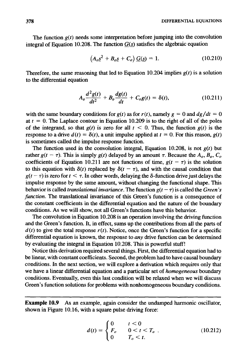
Figure
10.16
Undamped
Harmonic
Oscillator with
Square
Pulse
Drive
The nonhomogeneous differential equation describing the motion is
Md2
+
K,x(t)
=
d(t).
(10.213)
As
usual, we will assume that there is no response before the drive, and impose the
boundary conditions
x
=
0
and
dx/dt
=
0
at
t
=
0.
The first step in solving a problem of
this
type
is
to
determine the Green's function.
This
is done by solving the equation
+
K,g(t
-
T)
=
6(t
-
T),
Md2g:tl
T,
(10.214)
with the same type of boundary conditions:
g(t-T)=O t<T
=o
t<T.
(10.215)
dg(t
-
7)
dt
Applying a Laplace transform to
both
sides of Equation 10.214 gives
(MS*
+
K,)G(s,T)
=
e-ST,
(10.216)
where
G(s,
7)
is the Laplace transform of
g(t
-
7).
This
equation can be solved for
-
G(g,
7)
and then Laplace inverted to give the Green's function
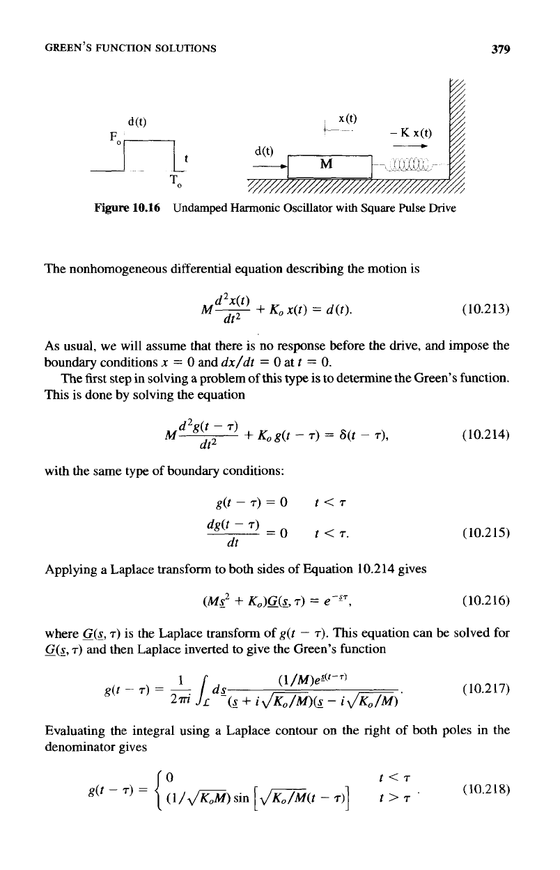
(10.2 17)
1 (1
/M)eX(('-')
(s
+
iJZZ%
-
iJKa/M)'
g(t
-
7)
=
g
LdS
Evaluating the integral using a Laplace contour on the right
of
both poles in the
denominator gives
380
DIFFERENTIAL
EQUATIONS
I
i
2
TO
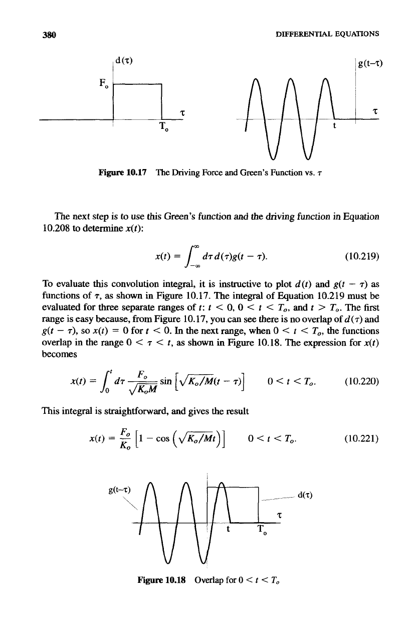
Figure
10.17
The
Driving
Force
and
Green’s
Function
vs.
7
The next step is
to
use
this
Green’s
function and the driving function in Equation
10.208
to determine
x(t):
x(t)
=
dTd(T)&
-
7).
(10.2
19)
To
evaluate
this
convolution integral, it
is
instructive to plot
d(t)
and
g(t
-
T)
as
functions of
T,
as
shown
in
Figure
10.17.
The integral of Equation
10.219
must be
evaluated for
three
separate ranges
of
I:
t
<
0,
0
<
t
<
To,
and
r
>
To.
The
first
range
is
easy because, from Figure
10.17,
you can
see
there is
no
overlap of
d
(
T)
and
g(t
-
T),
so
x(t)
=
0
for t
<
0.
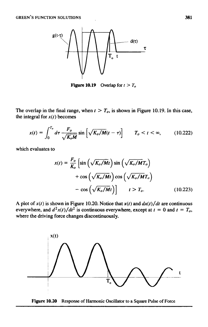
In
the next range, when
0
<
t
<
To,
the functions
overlap in
the
range
0
<
T
<
t,
as
shown
in
Figure
10.18.
The expression for
x(t)
becomes
1:
sin
[
dm(t
-
T)]
0
<
f
<
To.
(10.220)
This integral is straightforward, and gives the result
x(t)
=
3
[l
-
cos
(dst)]
0
<
t
<
To.
KO
(10.221)
Figure
10.18
Overlap
for
0
<
t
<
To
GREEN’S
FUNCTION
SOLUTIONS
381
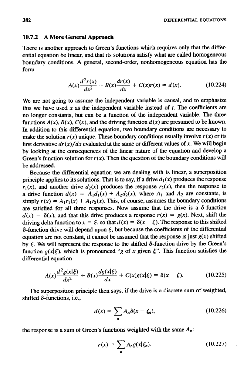
Figure
10.19
Overlap for
t
>
To
The overlap in the final range, when
t
>
To,
is shown in Figure
10.19.
In this case,
the integral for
x(t)
becomes
which evaluates to
-
cos
(JGt)]
t
>
To.
(10.223)
A
plot
of
x(t)
is shown in Figure
10.20.
Notice that
n(t)
and
dx(t)/dt
are continuous
everywhere, and
d2x(t)/dt2
is continuous everywhere, except at
t
=
0
and
t
=
To,
where the driving force changes discontinuously.
Figure
10.20
Response
of
Harmonic Oscillator to a Square
Pulse
of
Force
382
DIFFERENTIAL
EQUATIONS
10.7.2
A
More
General
Approach
There is another approach to Green’s functions which requires only that the differ-
ential equation
be
linear, and that its solutions satisfy what are called homogeneous
boundary conditions.
A
general, second-order, nonhomogeneous equation has the
form
d2r(x)
+
B(x)*
+
C(x)r(x)
=
d(x).
A(x)F dx
(10.224)
We are not going to assume the independent variable is causal, and to emphasize
this
we have used
x
as the independent variable instead of
f.
The coefficients are
no longer constants, but can be a function of the independent variable. The three
functions
A(x),
B(x),
C(x),
and the driving function
d(x)
are presumed to
be
known.
In
addition to
this
differential equation,
two
boundary conditions are necessary to
make the solution
r(x)
unique. These boundary conditions usually involve
r(x)
or its
first derivative
dr(x)/dx
evaluated at the same or different values of
x.
We will begin
by looking at the consequences of the
linear
nature of the equation and develop a
Green’s function solution for
r(x).
Then the question of the boundary conditions will
be addressed.
Because the differential equation we are dealing with is linear, a superposition
principle applies to its solutions. That is
to
say, if a drive
dl
(x)
produces the response
rl(x),
and another drive
dz(x)
produces the response
rz(x),
then the response to
a drive function
d(x)
=
Aldl(x)
+
A&$$),
where
A1
and
A2
are constants,
is
simply
r(x)
=
Alrl(x)
+
Alrz(x).
This,
of course, assumes the boundary conditions
are satisfied for all three responses. Now assume that the drive is a &function
d(x)
=
6(x),
and that
this
drive produces a response
r(x)
=
g(x).
Next, shift the
driving delta function to
x
=
E,
so
that
d(x)
=
6(x
-
6).
The response to
this
shifted
&function drive will depend upon
5,
but because the coefficients of the differential
equation are not constant, it cannot be assumed that the response is just
g(x)
shifted
by
6.
We will represent the response to the
shifted
6-function drive by the Green’s
function
&It),
which is pronounced
“g
of
x
given
e.
This
function satisfies the
differential equation
+
B(x)%
+
C(x)g(xlt)
=
6(x
-
6).
dx
(10.225)
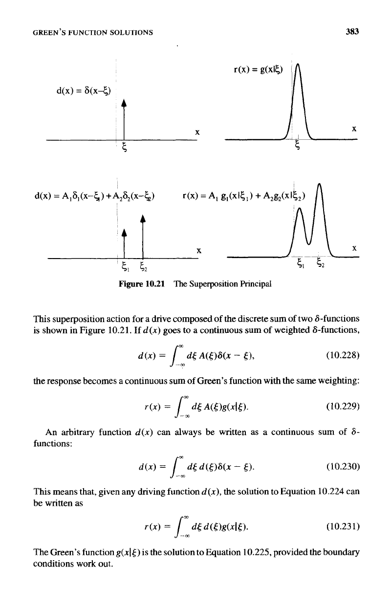
The superposition principle then says,
if
the drive is a discrete sum
of
weighted,
shifted &functions, i.e.,
the response is a sum of Green’s functions weighted with the same
An:
(10.226)
GREEN’S
FUNCTION
SOLUTIONS
383
t
X
This superposition action for a drive composed
of
the discrete sum of two &functions
is shown in Figure 10.21. If
d(x)
goes to a continuous sum of weighted &functions,
(10.228)
the
response becomes a continuous sum
of
Green’s function with the same weighting:
(10.229)
An
arbitrary function
d(x)
can always be written as a continuous sum
of
6-
functions:
(10.230)
This means that, given any driving function
d(x),
the solution to Equation 10.224 can
be written as
(10.231)
The Green’s function
g(x16)
is the solution to Equation 10.225, provided the boundary
conditions work out.
384
DIFFERENTIAL
EQUATIONS
Equation 10.225 cannot
be
solved for the Green’s function without specifying
boundary conditions for
g(x15).
Therefore, to obtain the Green’s function and eval-
uate the response in terms of the Green’s function integral of Equation 10.231, the
boundary conditions for
&It)
must
be
determined
so
that Equation 10.231 pro-
duces
an
r(x)
that still satisfies the original boundary conditions of the problem. Zero
boundary conditions on
r(x)
are
easy
to handle. By zero boundary conditions
we
mean that
r(x)
or a derivative of
r(x)
is zero at some value of
x,
say
x
=
x,.
If
this
is
the case, these boundary conditions on
r(x)
will be established by a Green’s function
that obeys the same boundary conditions, that
is
g(x15)
or its derivative is zero at the
same
x
=
x,,
for any
5.
These zero boundary conditions are specific examples of
homogeneous boundary conditions, which are discussed below,
list
for the specific
case of a second-order differential equations, and then
in
the general case.
For a second-order linear differential equation, two boundary conditions must
be
specified. They generally involve the response andor its first derivative, evaluated at
the same or
two
different values of the independent variable. The most general
forms
for homogeneous boundary conditions for a second-order equation are
(10.232)
(10.233)
where
a1,
a2,
PI
and
pZ
are constants.
If
these types of boundary conditions are
applied to a
&I[),
it
is easy to show that the
r(x)
generated by Equation 10.227,
and consequently Equation 10.231, will satisfy the same homogeneous boundary
conditions. The homogeneous boundary conditions of the Laplace Example
10.9
fit
thisformwitha=b=O,al =&=lranda2=P1=O.
For a linear, nonhomogeneous differential equation of
nth
order, there must be
n
boundary conditions that may involve the response up
to
its
n
-
1 derivative. For
an
nth-order equation, the general form of the homogeneous boundary conditions are
n
different equations:
di-’
r
(x)
2
air
=
0.
i=l
(10.234)
The first equation involves a set
of
constants
ai
and the function andor its derivatives
are evaluated at
x
=
a;
the second, a set of constants
pi
and terms evaluated at
x
=
b;
etc.
The Green’s function argument is now complete. Given a linear, nonhomogeneous
differential equation
in
the form of Equation 10.224 and a complete set
of
homo-
geneous boundary conditions in the form of Equation 10.234, the response can be
obtained from a Green’s function integral. The Green’s function
g(x15)
is the solution
to the original differential equation with a &function drive and satisfies the same set
of
homogeneous boundary conditions.
GREEN’S
FUNCTION SOLUTIONS
3885
This derivation for the Green’s function solution is correct, but a little sloppy.
In Appendix
D
there
is
a more formal, but far less intuitive proof for the existence
of Green’s functions and for the properties
of
homogeneous boundary conditions.
These proofs are for second-order differential equation, but are easily extended to
linear equations
of
any order.
~ ~ ~~ ~~ ~ ~~ ~ ~ ~ ~~~
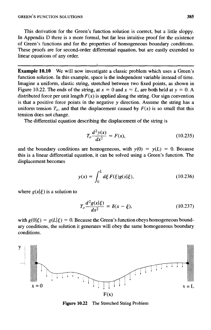
Example
10.10
We will now investigate a classic problem which uses a Green’s
function solution. In this example, space is the independent variable instead of time.
Imagine a uniform, elastic
string,
stretched between two fixed points, as shown in
Figure 10.22. The ends of the string, at
x
=
0
and
x
=
L,
are both held at
y
=
0.
A
dlstributed force
per
unit length
F(x)
is applied along the string. Our sign convention
is that a positive force points in the negative
y
direction. Assume the string has a
uniform tension
To,
and that the displacement caused by
F(x)
is
so
small that this
tension does not change.
The differential equation describing the displacement of the string is
(10.235)
and the boundary conditions are homogeneous, with
y(0)
=
y(L)
=
0.
Because
this is
a
linear differential equation, it can
be
solved using a Green’s function. The
displacement becomes
where
g(x16)
is
a solution to
(10.236)
(10.237)
with
g(O16)
=
g(L16)
=
0.
Because the Green’s function obeys homogeneous bound-
ary
conditions, the solution it generates will obey the same homogeneous boundary
conditions.
F(x)
Figure
10.22
The
Stretched
String
Problem