Kusse B.R., Westwig E.A. Mathematical Physics: Applied Mathematics for Scientists and Engineers

3%

DIFFERENTIAL EQUATIONS

The Green’s function for this problem is the response of the rod to a &function

impulse at position

x

=

5

and time

t

=

7.

It obeys the partial differential equation:

(10.281)

The homogeneous boundary conditions

T(x,

1)

must satisfy are also applied to the

Green’s function,

so

g(x15,rlT)

--$

0

as

x

+

tw.

The causality condition requires

that

g(x15,?1T)

=

0

for

t

<

T.

To

solve Equation 10.281, we will take a Fourier

transform in space, and a Laplace transform in time. Taking these transforms of the

Green’s function in two steps gives

G&$.tIT)

=

-

hg(xlt,

tlr)e-ib (10.282)

i&L(klSr&)

=

1

dtG&15,t1T)e-”.

(10.283)

The Fourier-Laplace transform of Equation 10.281, the original differential equation,

gives the algebraic relation

m

(10.284)

This allows

us

to

solve for the Fourier-Laplace transform of the Green’s function

(10.285)

Now

all that remains

to

obtain the Green’s function is the double inversion

of

Equation 10.285. In principle, the inversions could be done in either order. In this

case, it is much easier to

do

the Laplace inversion

first.

The Laplace inversion can

be

evaluated from

(10.286)

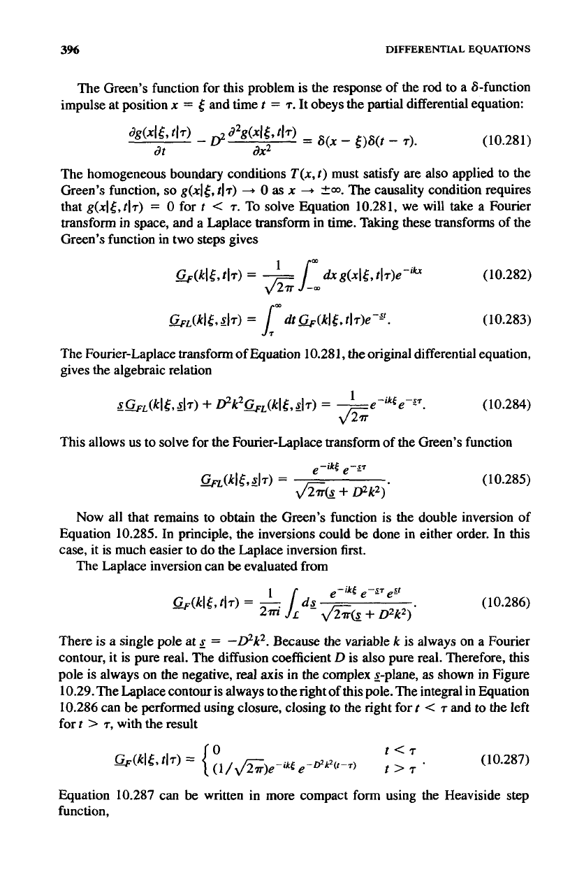
There

is

a single pole at

g

=

-dk2.

Because the variable

k

is always on a Fourier

contour, it is pure real. The diffusion coefficient

D

is also pure real. Therefore, this

pole is always on the negative, real axis in the complex g-plane,

as

shown in Figure

10.29. The Laplace contour

is

always to the right of this pole. The integral in Equation

10.286 can be performed using closure, closing to the right

for

t

<

7

and to the left

fort

>

T,

with the result

(10.287)

Equation 10.287 can be written in more compact form using the Heaviside step

function,

IOUNDARY CONDlTIONS

imag

397

db

L

real

___c__

-

DZk2

?gum

10.29

Laplace

Inversion

for

the

Nonhomogeneous

Diffusion Equation Green’s

Func-

ion

0

t<7

1

f>T’

H(t

-

T)

=

1s

(10.288)

(10.289)

The space-time Green’s function is now obtained by applying a Fourier inversion to

Quation

10.289:

(10.290)

he way to solve this integral is by completing the square of the integrand’s exponent.

Instead, we will use the convolution trick again. Notice the function in Equation

10.289

can

be

written as the product of

two

functions:

(10.291)

Zonsequently, the Green’s function

can

be

written

as

1/&

times the convolution

xer

x

of their inverse transforms:

398

DIFFERENTIAL

EQUATIONS

i

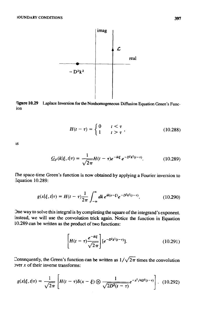
g(

Figure

10.30

Green's

Function

for

the Diffusion

Equation

with

a

Distributed

Heat

Source

Because

of

the 6-function,

this

convolution easily evaluates to

(10.293)

A

plot

of

this

Green's function

is

shown

in

Figure

10.30.

There

are

some interesting things

to

notice about this Green's function.

First,

the

tlr

dependence has

the

form

t

-

T

and the

XI(

dependence has the

form

x

-

5.

These

results make sense both mathematically and physically. Mathematically,

this

occurs

because the problem

has

constant coefficients and homogeneous boundary conditions

at

x

=

30.

Physically, it

is

clear from symmetry, the problem must

be

translationally

invariant in both time and space.

Also

notice there

is

a symmetry with respect

to

the

x

and

6

variables, with

g(x15,

tl~)

=

g(fln,

tIT),

while there

is

no

such symmetry

for

the

t

and

T

variables,

g(xl(,

t17)

f

?g(xl(,

dr).

This symmetry property will

be

explored in one

of

the exercises at the end of

this

chapter.

~~~

Example

10.13

As

a

final

example, the Green's function for a driven wave

equation

will

be

developed.

The

one-dimensional driven wave equation

for

propagation

in

a

BOUNDARY

CONDITIONS

399

uniform medium can be written as

1

d2U(X,t)

82u(x,t)

c;

dt2

8x2

=

s(x,

t).

(10.294)

The constant

c,

is the velocity of propagation of the wave.

This

is a nonhomogeneous

equation, with the response

u(x,

t)

generated by the distributed source term

s(x,

t).

This problem can be treated with a spatial Fourier transform and a temporal

Laplace transform, exactly like the diffusion equation of the previous example. There

is no problem with this approach. We will demonstrate a different approach, however,

because it is one commonly used in physics calculations.

To

avoid the tedious Laplace

transform, we will assume that the time behavior

of

both the driving term and the

response are in the

sinusoidal steady state,

so

all the time dependence occurs with a

constant amplitude at a fixed frequency

a,.

In

other words, we assume that

s(x,t)

=

Real

[S(x)eimo']

,

(10.295)

and the response has a similar time dependence

u(x,t)

=

Real

[U(x)eimo']

.

(10.296)

As

you will see, this is very much like taking a Fourier transform in time. Unfortu-

nately, you will also find out it presents a few problems!

In this sinusoidal steady state, the differential equation becomes

0,'

d2U4

-

U(x)

-

=

$(x).

c;

-

dx2

(10.297)

Notice the time dependence completely cancels out, and we have a linear, nonhomo-

geneous equation for

U(x).

Also,

we now are dealing with only a single independent

variable,

so

the partial derivative

has

been replaced by a regular derivative. The

solution for

_U(x)

can be formulated in terms of a Green's function,

where

g(x16)

satisfies the differential equation

We can take the Fourier transform of both sides of this equation to give

(10.298)

(10.299)

(10.300)

400

DIFFERENTIAL EQUATIONS

~

IFbg=

_real

Figure

1031

Fourier Inversion

for

the Driven Wave

Equation

so

that

(10.301)

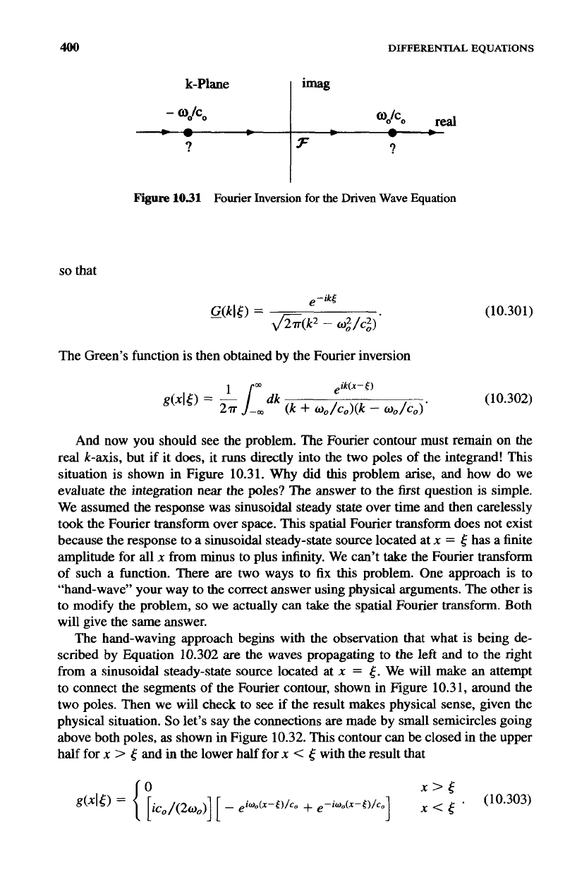
The Green’s function is then obtained by the Fourier inversion

And now you should see the problem. The Fourier contour must remain on the

real

k-axis,

but

if

it does, it

runs

directly into the

two

poles

of

the integrand!

This

situation is shown in

Figure

10.31. Why did

this

problem arise, and how do we

evaluate the integration near the poles? The answer to the

first

question is simple.

We assumed the response was sinusoidal steady state over time and then carelessly

took the Fourier transform over space.

This

spatial Fourier transform does not exist

because the response to a sinusoidal steady-state source located at

x

=

5

has a finite

amplitude for

all

x

from minus to plus infinity. We can’t

take

the Fourier transform

of

such a function. There

are

two ways to

fix

this

problem. One approach is to

“hand-wave” your way to

the

correct answer using physical arguments. The other is

to modify the problem,

so

we actually can take the spatial Fourier transform. Both

will give the

same

answer.

The hand-waving approach begins with the observation that what is being de-

scribed by Equation 10.302

are

the waves propagating

to

the

left

and to the right

from a sinusoidal steady-state source located at

x

=

5.

We will make an attempt

to connect the segments of the Fourier contour, shown in Figure 10.31, around the

two poles. Then we will check to see if the result

makes

physical sense, given the

physical situation.

So

let’s say the connections are made by small semicircles going

above both poles,

as

shown in Figure 10.32.

This

contour can

be

closed in the upper

half for

x

>

5

and in the lower half for

x

<

5

with the result that

(10.303)

BOUNDARY

CONDITIONS

401

X

-No

Response-

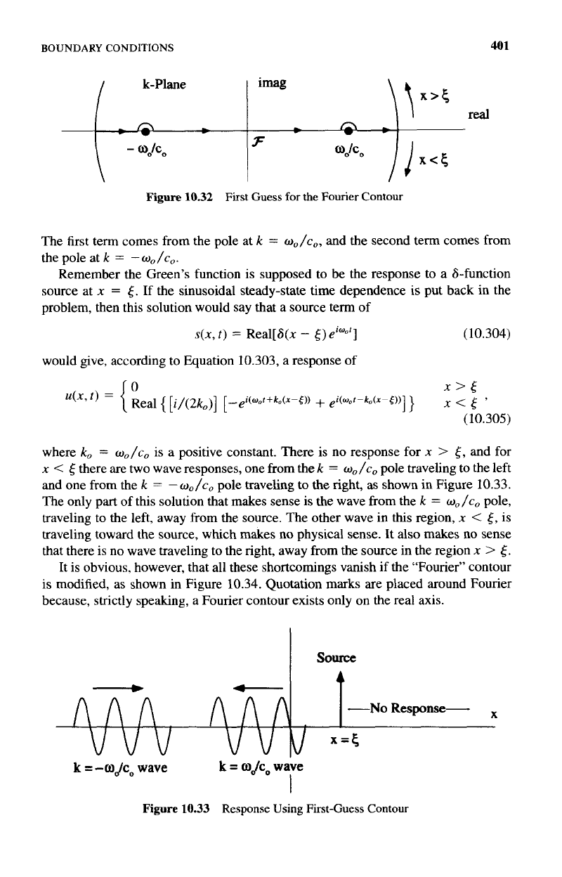
Figure

10.32

First Guess for the Fourier Contour

The first term comes from the pole at

k

=

wo/co,

and the second term comes from

the pole at

k

=

-

wo/co.

Remember the Green’s function is supposed to be the response to a &function

source at x

=

5.

If the sinusoidal steady-state time dependence is put back in the

problem, then this solution would say that a source term of

s(x,

t)

=

Real[S(x

-

5)

eioofl

(10.304)

would give, according to Equation 10.303, a response of

where

k,

=

w,/co

is

a positive constant. There

is

no response for x

>

5,

and for

x

<

5

there are two wave responses, one from the

k

=

wo/co

pole traveling to the left

and one from the

k

=

-wo/co

pole traveling to the right, as shown in Figure 10.33.

The only part of this solution that makes sense is the wave from the

k

=

wo/co

pole,

traveling to the left, away from the source. The other wave in this region,

x

<

5,

is

traveling toward the source, which makes

no

physical sense. It also makes no sense

that there is no wave traveling to the right, away from the source in the region x

>

5.

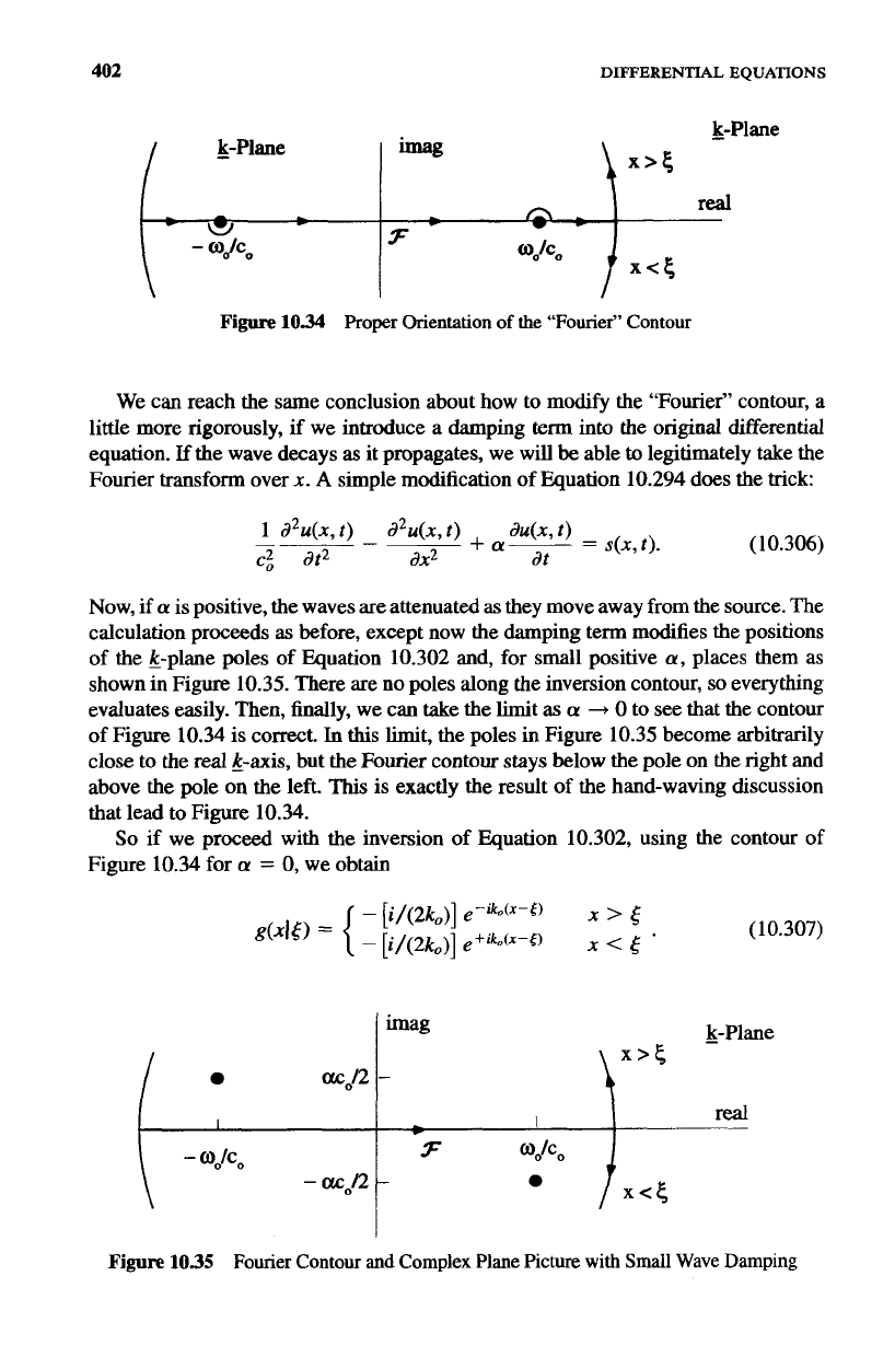
It is obvious, however, that

all

these shortcomings vanish if the “Fourier” contour

is modified, as shown in Figure 10.34. Quotation

marks

are placed around Fourier

because, strictly speaking, a Fourier contour exists only on the real axis.

Figure

10.33

Response Using

First-Guess

Contour

402

-

k-Plane

L

-

-w

-

OJCO

DIFFERENTIAL EQUATIONS

x>s

imag

real

-

OO’CO

3

x<5

We can reach the same conclusion about how to modLfy the “Fourier” contour, a

little more rigorously,

if

we introduce a damping

krm

into the original differential

equation.

If

the wave decays

as

it propagates, we

will

be able to legitimately take the

Fourier transform over

x.

A

simple modification of Equation

10.294

does the trick

(10.306)

1

d2U(X,t)

du(x

t)

c;

at2

dX2

dt

+

a2

=

s(x,t).

Now, if

a!

is positive, the waves are attenuated

as

they move away from the source. The

calculation proceeds

as

before, except now the damping term modifies the positions

of the &plane poles

of

Equation

10.302

and, for small positive

a,

places them

as

shown in Figure

10.35.

There are no poles along the inversion contour,

so

everything

evaluates easily. Then, finally, we can take the limit

as

a

+

0

to see that the contour

of Figure

10.34

is

correct.

In

this

limit, the poles

in

Figure

10.35

become arbitrarily

close to the real &axis, but the Fourier contour stays

below

the pole on the right

and

above the pole on the left.

This

is exactly the result of the hand-waving discussion

that lead to Figure

10.34.

So

if

we proceed with the inversion

of

Equation

10.302,

using the contour of

Figure

10.34

for

a!

=

0,

we obtain

(1

0.307)

acJ2

1.

imag k-Plane

Figure

1035

Fourier

Contour

and

Complex Plane Picture with Small Wave Damping

BOUNDARY

CONDITIONS

403

1

Source

f--

't

-

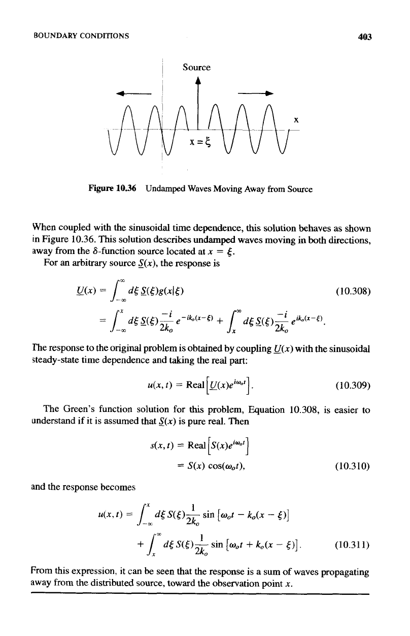
Figure

10.36

Undamped

Waves

Moving

Away

from

Source

When coupled with

the

sinusoidal time dependence,

this

solution behaves as shown

in Figure 10.36.

This

solution describes undamped waves moving in both directions,

away from the &function source located at

x

=

5.

For an arbitrary source

S(x),

the response

is

(10.308)

me response to the original problem

is

obtained

by

coupling

_U(x)

with the sinusoidal

steady-state time dependence and taking the real part:

u(x,t)

=

Real

_U(x)eiWo'

.

(10.309)

The Green's function solution for

this

problem, Equation

10.308,

is easier to

[I

understand if it is assumed that

S(x)

is pure real. Then

s(n,t)

=

Real

S(x)eiwo'

11

=

S(X)

cos(o,t), (10.310)

and the response becomes

(10.311)

From this expression, it can be seen that the response is a sum of waves propagating

away from the distributed source, toward

the

observation point

x.

1.

+

Lrn

4

stoz

[coot

+

ko(n

-

5)].

404

DIFFERENTIAL

EQUAlTONS

EXERCISES FOR CHAPTER

10

1.

Determine whether the following differential equations are homogeneous or

nonhomogeneous, and linear

or

nonlinear:

2.

The rate of evaporation for a constant-density, spherical drop is proportional

to its surface area. Assume

this

evaporation is the only way the drop can lose

mass

and detennine a differential equation that describes the time dependence

of

the

radius

of the drop. Solve

this

equation for the radius

as

a function of time,

assuming that at

t

=

0

the radius is

r,.

3.

Using separation of variables, solve the differential equation

dyo

22

=xy,

dx

with the boundary condition

y(0)

=

5.

What happens when you

try

to impose

the boundary condition that

y(0)

=

O?

4.

Consider the differential equation

dY(X)

- -

y

dx

X’

with the boundary condition

y(

1)

=

1.

(a)

Solve

this

equation using separation of variables.

(b)

This

equation can also be solved

by

converting it into an exact differential.

Using the notation of Equations

10.21-10.24,

identify the functions

R(x,

y),

S(x,

y),

and

4(x,

y).

Using the boundary condition, find a solution

#(x,

y)

=

C,

that is equivalent to your answer in

part

(a).

5.

Consider the differential equation

dyo

YG)

+

-

=

cos(x2).

dx

X

(a)

Determine an integrating factor for

this

equation.

(b)

Solve for

y(x).

EXERCISES

405

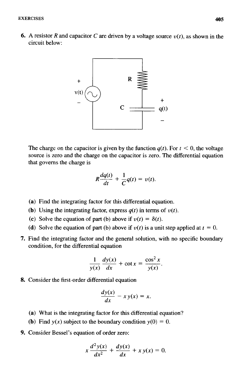
6.

A

resistor

R

and capacitor

C

are driven by a voltage source

v(t),

as shown in the

circuit below:

The charge on the capacitor is given by the function

q(t).

For

t

<

0,

the voltage

source is zero

and

the charge on the capacitor is zero. The differential equation

that governs the charge

is

1

R-

+

-q(t)

=

v(t).

dt

C

(a)

Find the integrating factor for this differential equation.

(b)

Using the integrating factor, express

q(t)

in terms of

v(t).

(c)

Solve the equation of part (b) above if

v(t)

=

&t).

(d)

Solve the equation

of

part (b) above

if

v(t)

is a unit step applied at

t

=

0.

7.

Find the integrating factor and the general solution, with no specific boundary

condition, for the differential equation

8.

Consider the first-order differential equation

(a)

What is the integrating factor for

this

differential equation?

(b)

Find

y(x)

subject to the boundary condition

y(0)

=

0.

9.

Consider Bessel’s equation of order zero:

d2Y(X)

x

-

+

xy(x)

=

0.

dx2 dx

Kusse B.R., Westwig E.A. Mathematical Physics: Applied Mathematics for Scientists and Engineers

Подождите немного. Документ загружается.