Kusse B.R., Westwig E.A. Mathematical Physics: Applied Mathematics for Scientists and Engineers
Подождите немного. Документ загружается.

386
DIFFERENTIAL EQUATIONS
x=L
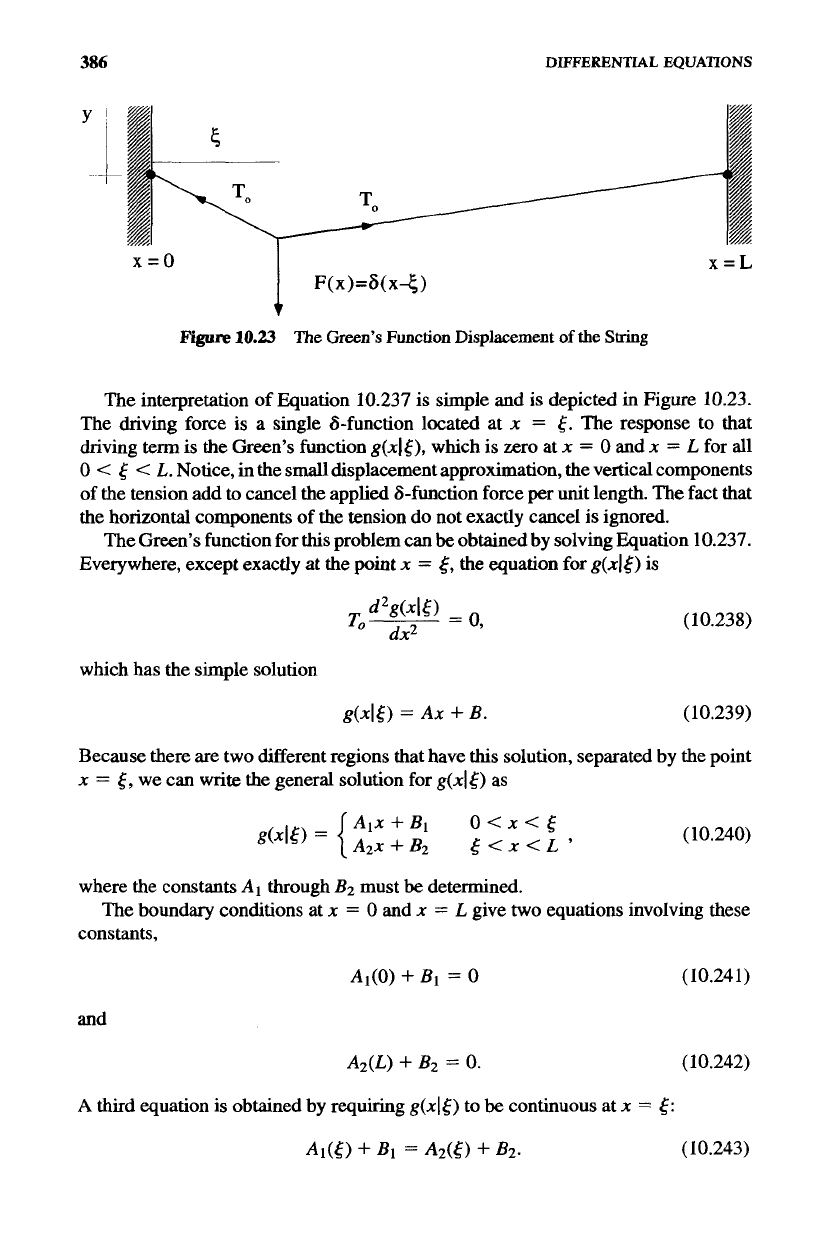
Figure
10.23
The
Green’s
Function
Displacement
of
the
String
The interpretation of Equation 10.237 is simple and is depicted in Figure 10.23.
The driving force is a single 6-function located at
x
=
6.
The response to that
driving
term
is
the Green’s function
&It),
which is zero at
x
=
0
and
x
=
L
for all
0
<
5
<
L.
Notice,
in
the small displacement approximation, the vertical components
of the tension add to cancel the applied 6-function force per
unit
length. The fact that
the horizontal components of the tension do not exactly cancel is ignored.
The Green’s function for
this
problem can
be
obtained by solving Equation 10.237.
Everywhere, except exactly
at
the
point
x
=
6,
the equation for
g(x15)
is
(10.238)
which
has
the simple solution
g(x15)
=
Ax
+
B.
(10.239)
Because there are two different regions that have
this
solution, separated by the point
x
=
6,
we
can write the general solution for
g(x16)
as
(10.240)
where the constants
A1
through
B2
must
be
determined.
constants,
The boundary conditions at
x
=
0
and
x
=
L
give
two
equations involving these
Al(0)
+
B1
=
0
(10.241)
and
A2(L)
+
B2
=
0.
(10.242)
A
third equation is obtained by requiring
&I[)
to
be
continuous at
x
=
6:
A]([)
+
BI
=
A2(6)
+
B2.
(10.243)
BOUNDARY CONDITIONS
387
In other words, the string does not break due to
the
force. The fourth and final equation
takes a bit more work, and involves the driving term
6(x
-
0,
which has not yet been
used. Start by integrating Equation 10.237 from
x
=
5
-
E
to
x
=
5
+
E
in the limit
of
E
--+
0:
(
10.244)
The
LHS
of
this
equation goes to
To
times the discontinuity in slope of
g(xl5)
at
x
=
6,
and the
RHS
is one because we
are
integrating over a &function. The result
is
(10.245)
Taking the limit as
E
+
0,
and referring back to Equation 10.240, gives
To
(A2
-
Al)
=
1. (10.246)
Notice that this equation is essentially a statement that the vertical forces at
x
=
5
must cancel. Equations 10.241-10.243, along with Equation 10.246, constitute a set
of four independent equations that uniquely determine
Al, A2,
B1,
and
Bz.
Equation
10.240 for the Green’s function becomes
Notice that this Green’s function does not have the simple form
g(x
-
5)
of a
translationally invariant solution.
A
quick look at Figure 10.23 and the boundary
conditions at the ends of the string show why
this
must be the case.
This Green’s function can now be used in Equation 10.236 to obtain the displace-
ment
of
the string for an arbitrary loading force density
F(x).
Some care, however,
must be taken in setting up
this
integral. For
this
integration,
x
is held fixed, some-
where between
0
and
L,
while the integration variable
5
ranges from
0
to
L.
According
to Equation 10.247,
g(x15)
=
g2(x15)
when
5
<
x
and
=
g1(x15)
when
5
>
x.
The integration of Equation 10.236 must therefore be broken up into two parts. The
Green’s function solution for an arbitraxy
F(x)
becomes
10.7.3
Nonhomogeneous
Boundary
Conditions
Up to now, the Green’s function analysis has been for problems with homogeneous
boundary conditions. In this section, we will review, briefly, why homogeneous
388
DIFFERENTIAL
EQUATIONS
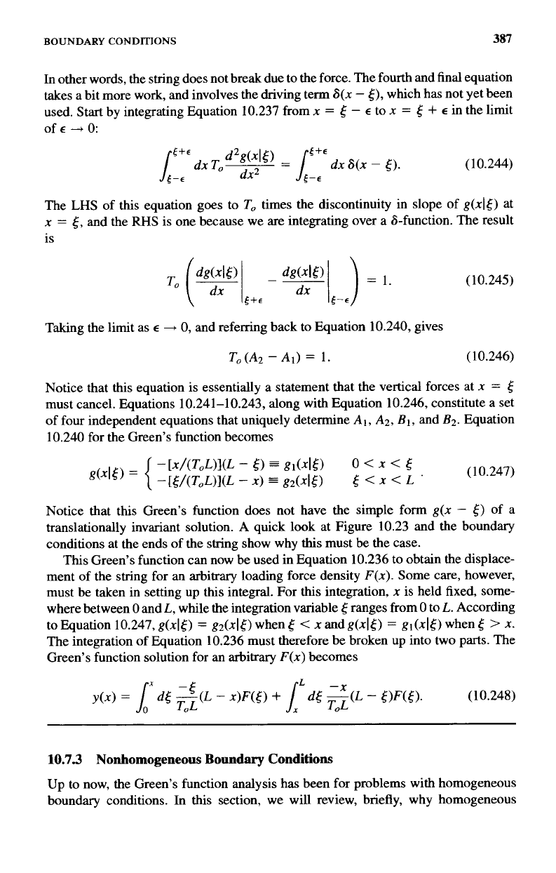
Figure
10.24
Homogeneous
Boundary Conditions
boundary conditions are important. Then a method for dealing with nonhomogeneous
boundary conditions will be introduced.
In
the case
of
the stretched string problem, the example of the previous section,
the homogeneous boundary conditions specified that the response be zero at either
end
of
the string. These boundary conditions
fit
the general homogeneous form
of Equation 10.234. We
required
the Green’s function to obey the
same
boundary
conditions.
This
works because when the Green’s function is constrained to be zero
at
x
=
0
and
x
=
L,
as shown
in
Figure 10.23, an arbitrary
sum
of Green’s functions
will
automatically obey the same conditions.
As
an example of
this,
the
sum
of
three Green’s functions is depicted
in
Figure 10.24. Therefore, forcing the Green’s
function to obey the same boundary conditions as the original differential equation
is the proper approach
in
this
case.
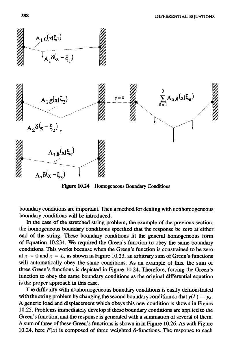
The difficulty with nonhomogeneous boundary conditions is easily demonstrated
with the string problem by changing the second boundary condition so that
y(L)
=
yo.
A
generic load and displacement which obeys
this
new condition is shown
in
Figure
10.25. Problems immediately develop
if
these
boundary
conditions are applied
to
the
Green’s function, and the response is generated with a summation
of
several
of
them.
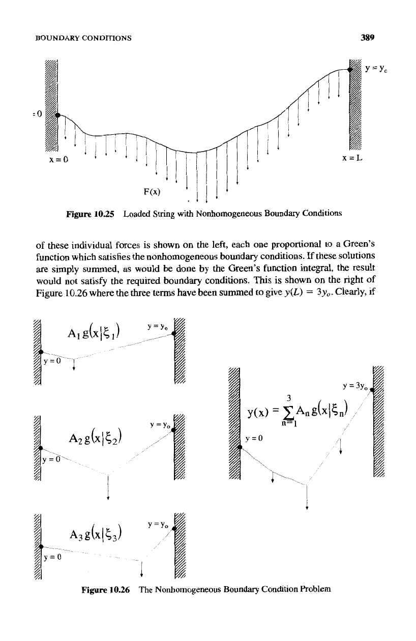
A
sum of
three
of
these Green’s functions is shown
in
in Figure 10.26.
As
with Figure
10.24, here
F(x)
is composed of three weighted 6-functions. The response to each
BOUNDARY
CONDITIONS
389
Y
=
Yo
=O
Figure 10.25
Loaded
String
with
Nonhomogeneous
Boundary
Conditions
of these individual forces is shown on the left, each one proportional to a Green’s
function which satisfies the nonhomogeneous boundary conditions.
If
these solutions
are simply summed, as would be done by the Green’s function integral, the result
would not satisfy the required boundary conditions.
This
is
shown on the right
of
Figure
10.26
where the three terms have been summed to give
y(L)
=
3y0.
Clearly, if
Y
=Y
_,
~.~
Y=
,/’
i
-
The
Nonhomogeneous Boundary
Condition
Problem
Y=3Y
5,)
I
390
DIFFERENTIAL
EQUATIONS
g(x16)
satisfies the nonhomogeneous boundary conditions, the correct answer is not
generated by the Green’s function
sum.
Fortunately, there is a way around
this
problem. It
is
clear
from
the picture above
that to keep the generic Green’s function integral
(10.249)
from diverging for
n
=
a
or
x
=
b,
the Green’s function must be forced to have
homogeneous boundary conditions. But we can add
to
this
function another
term,
which makes the solution obey the nonhomogenwus boundary conditions.
To
see how
this
works, let’s
return
to the string problem with the nonhomogeneous
boundary conditions
y(0)
=
0
and
y(L)
=
yo.
The solution
y(x)
still satisfies the
differential equation
d2Y(X>
To-
=
F(x).
dx2
(10.250)
Now break
y(x)
into two parts,
Y(4
=
YlW
+
y2(x),
(10.25 1)
where
y1
(x)
satisfies the nonhomogeneous differential equation, Equation 10.250,
but has homogeneous boundary conditions, i.e.,
yl(0)
=
0
and
yl(L)
=
0.
Let
y2(x)
satisfy the homogeneous version
of
Equation 10.250
(10.252)
with the nonhomogeneous boundary conditions,
y2(0)
=
0
and
y2(L)
=
yo.
The
sum of these two solutions,
yl(x)
+
y2(x),
will satisfy
both
the nonhomogeneous
differential equation
and
the nonhomogeneous boundary conditions. The
y1
(x)
part
of the solution can
be
found with the standard Green’s function approach, by requiring
the
Green’s function
to
satisfy homogeneous boundary conditions. The
y2(x)
part
is
obtained by solving
a
simple homogeneous differential equation and then applying
the nonhomogeneous boundary conditions.
In
this
case,
yl(x)
is
the same solution found
in
Equation
10.248:
L
(10.253)
Yl(4
=
[dSF(OG(L
-6
-
x)
+
J:
dtF(O&L
-
0.
The
y2(x)
part
of the solution, the solution to Equation 10.252, is simply
Y~(x)
=
AX
+
B.
(10.254)
Applying the nonhomogeneous boundary conditions forces the constants to be
A
=
yo/L
and
B
=
0,
so
that the total solution is
BOUNDARY CONDITIONS
391
--x
L
Y(X)
=
LxdSfWT,L(L
-5
-
x>
+
/
&F(~)T,L(L
-
0
+
(10.255)
~n
summary, to solve a linear, nonhomogeneous differential equation with non-
homogeneous boundary conditions, break the problem into two parts. Use a Green’s
function approach to solve the original, nonhomogeneous differential equation using
a Green’s function which satisfies homogeneous boundary conditions. The desired
solution is then the sum of
this
solution and the solution to a homogeneous version
of
the differential equation, which obeys the nonhomogeneous boundary conditions.
X
L
10.7.4
Multiple Independent Variables
To
this point, all our Green’s function examples have had a single independent vari-
able. How
are
things modified when we consider higher dimensions?
In
this
section,
through examples, we will explore two-dimensional solutions for two common prob-
lems, diffusion and wave propagation. Both examples have one space dimension and
the time dimension.
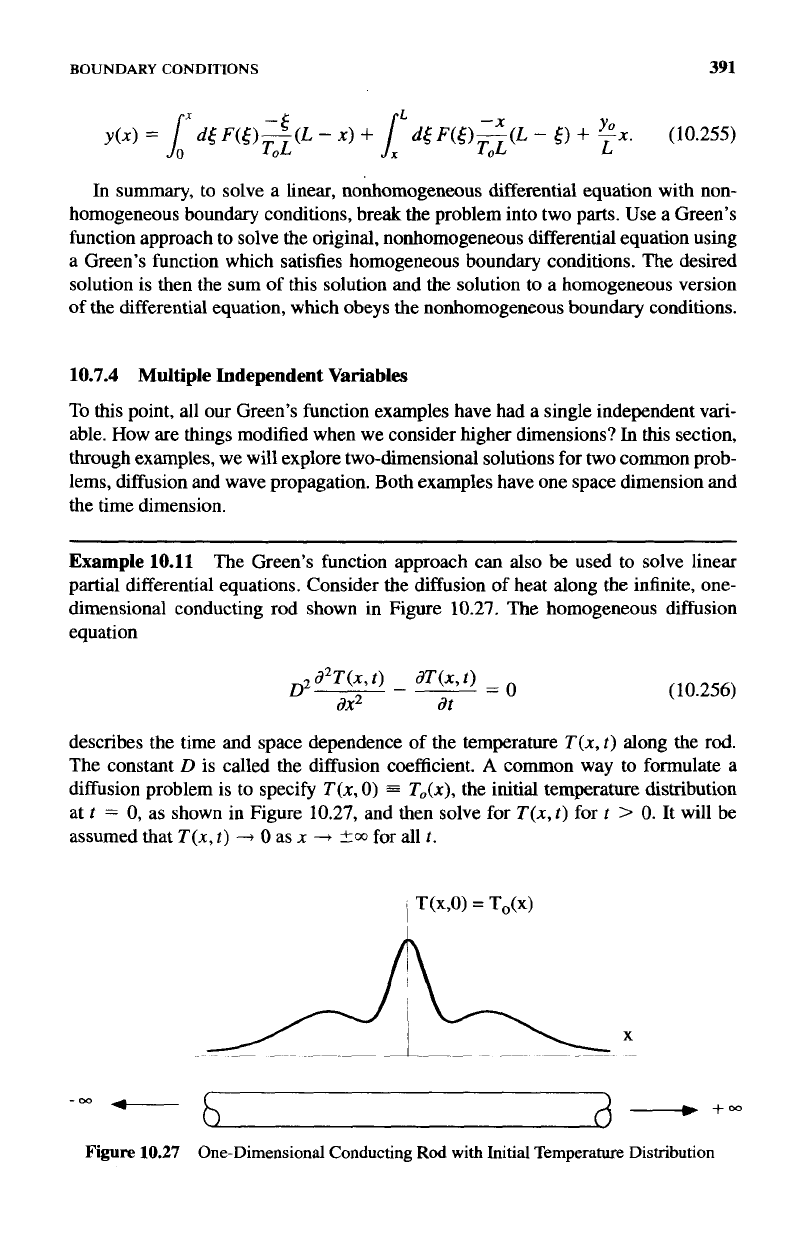
Example 10.11
The Green’s function approach can also
be
used to solve linear
partial differential equations. Consider the diffusion of heat along the infinite, one-
dimensional conducting rod shown in Figure
10.27,
The homogeneous diffusion
equation
dZT(x,
t)
dT(x,
t)
D2---
=o
ax*
at
(10.256)
describes the time and space dependence of the temperature
T(n,
t)
along the rod.
The constant
D
is called the diffusion coefficient.
A
common way to formulate
a
diffusion problem is
to
specify
T(x,
0)
=
T,(x),
the initial temperature distribution
at
t
=
0,
as shown in Figure
10.27,
and then solve for
T(x,
t)
for
t
>
0.
It will be
assumed that
T(x,
t)
-+
0
as
x
+
503
for all
t.
-b
d-+-
-w
Figure
10.27
One-Dimensional
Conducting
Rod
with
Initial
Temperature Distribution
392
DIFFERENTIAL
EQUATIONS
At first, this does not look like a problem that could be solved using a Green’s
function method, since the differential equation is homogeneous and there
is
no
driving term. It
is,
however, a linear equation,
so
the superposition principle does
apply. That is to say, if
To(x)
=
6(x
-
5)
results in
T(x,
t)
=
g(x15,
t),
then
TAX)
=
C
AnNx
-
en)
(10.257)
n
will result in
(10.258)
n
for
all
t
>
0.
Taking these summations to continuous integrals allows us to argue
that, if
T&)
=
Srn
d5
To(S)&
-
51,
(10.259)
--m
then
(10.260)
for all
t
>
0.
Notice how we have set up the arguments of the Green’s function. The
variables
x
and
6
have been used as
standard
Green’s function variables, while
t
is
not involved in the Green’s function integral of Equation 10.260.
This
is indicated by
the notation in the argument of the Green’s function. Only variables immediately to
the right of a
“I”
will take part in Green’s function integrations.
So
the solution to the problem can be formulated using a Green’s function, with
the initial temperature distribution acting
as
the weighting function in the Green’s
function integral. The boundary conditions require
T(x,
I)
-t
0
as
x
-+
+co
and are
homogeneous. Consequently, the
same
boundary conditions are applied to
g(x15,
t).
This
Green’s function must satisfy
(10.261)
with the initial condition at
I
=
0
g(xl6,O)
=
6(x
-
5)
(10.262)
and the boundary conditions described above. Notice
in
this
problem, the
initial
condition is treated very differently
from
the boundary conditions.
One method to solve Equation 10.261 is to use a Fourier transform in space.
A
standard Laplace transform cannot be used because the solution must be valid for
all
x.
We define
-
G(k(6,t)
-
1:
dxg(X15,
t)e-ik“,
(
10.263)
BOUNDARY
CONDITIONS
md the Fourier transform of Equation 10.261 becomes
393
(10.264)
This is
an
easy first-order equation, with the general solution
-
G(k15,
t)
=
G-
ePdk2',
(10.265)
where the complex constant
G-
=
G(k15.0).
But
g(xl5,
0)
=
6(x
-
t),
so
G
=
3.'&15>0))
The Fourier transform of the Green's function becomes
(10.266)
(10.267)
md the Green's function, itself, is the Fourier inversion
of
this
expression:
1
s(xl57t)
=
-
dk
-e-ikte-dk2ter~
(10.268)
This inversion can be done most easily using a convolution trick. The Fourier
6-m
Irn
J2.rr
ransform of this Green's function can be
looked
at
as
the product of two functions
W15,
t)
=
F(k15,
t)Ll(k15.t>,
(10.269)
where
(10.270)
(10.271)
The Green's function is therefore
1/&
times the convolution of the Fourier
nversions of Equations 10.270 and 10.271. Convolution is usually a messy process,
wt not in this case because the inversion of 10.270 is just a &function
(10.272)
394
DIPFERENTlAL EQUATIONS
and 8-functions convolve easily. The second function, Equation 10.271,
is
a Gaussian
and it inverts to another Gaussian:
The Green’s function becomes a convolution over
x:
(10.273)
(10.274)
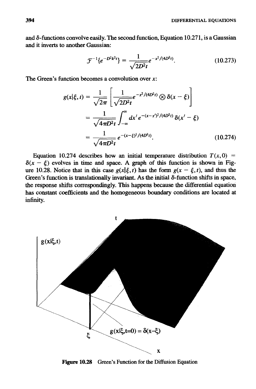
Quation 10.274 describes how an initial temperature distribution
T(x,O)
=
S(x
-
5)
evolves in time and space.
A
graph
of
this
function
is
shown
in Fig-
ure 10.28. Notice that
in
this
case
g(x16,t)
has
the
form
g(x
-
[,t),
and thus the
Green’s function
is
translationally invariant.
As
the initial 8-function
shifts
in space,
the response
shifts
correspondingly.
This
happens because the differential equation
has
constant coefficients and the homogeneous
boundary
conditions are located at
infinity.
Figure
10.28
Green’s
Function
for
the
Diffusion
Equation
BOUNDARY
CONDITIONS
395
The general response for an arbitrary initial temperature distribution
To(x)
is then
T(x,t)
=
-
d,$
To(,$)
e-(x-&2/(4dI)
(10.275)
Notice the integration of Equation 10.275 is over only the
x
variable. The
t
variable
just hangs around as a simple time dependence of the Green’s function.
In
the next
example, both time and space
are
treated as Green’s function variables, and the
response will involve
an
integral over both of these quantities.
Ja
Srn
--m
Example
10.12
We now consider the same one-dimensional, conducting rod as we
used in the previous example, but
this
time with an external driving term. Imagine a
special heating element, running
through
the
center of the rod, which can add heat in
an arbitrary way that depends both on
x
and
t.
The heat source
s(x,
t)
turns
Equation
10.256 into a nonhomogeneous differential equation:
(10.276)
The signs have been adjusted in
this
equation
so
that a positive source term produces
a positive change in temperature. The solution still must obey the homogeneous
boundary conditions,
T(x,t)
-+
0
as
x
+
fm.
In
addition, we will
also
assume
that
the
rod obeys causality with respect to the time variable. That is, there can be
no response in the rod before the heat source is applied. The source term
s(x,
t)
is
assumed to be zero for
t
<
0,
so
that
T(x,
t)
=
0
for
t
<
0.
Because Equation 10.276 is a linear equation with homogeneous boundary con-
ditions, it must obey the superposition principle. Thus, if a drive of
s(x,t)
=
S(x
-
,$)S(t
-
7)
results in
T(x,
t)
=
g(xI,$,
tIT),
then a drive of
nm
causes
a
temperature response
of
(10.278)
nm
This
reasoning can
be
extended for continuous quantities by converting the summa-
tions into integrals.
So
if the drive is now
s(x,
t)
=
1:
d5
1:
d7s(,$,
7)Wx
-
OW
-
4,
(10.279)
the response is
T(x,
t>
=
1:
d5
l:dTs(,$,
7)g(xI,$,
tb).
(10.280)