Kusse B.R., Westwig E.A. Mathematical Physics: Applied Mathematics for Scientists and Engineers
Подождите немного. Документ загружается.

426
SOLUTIONS
TO
LAPLACE’S
EQUATION
form of
@(x,
y.
z)
is constructed and initially just concentrate on the functional form
of the separated solutions. Equation 1
1.10
will
be written, using a shorthand notation,
as
X(x)
-+
{
e-&x
e+fix
c,
#
0.
(11.11)
We now turn
our
attention
to
the solutions for
X(x)
with different separation
constants. The constant
c,
may
be
negative and real, positive and
real,
or complex.
Because the solution depends on the square mot of
c,,
it turns out the results
of
a
complex
c,
are covered by a combination
of
solutions generated by real positive
c,
and real negative
c,.
Thus, we
will
limit
our
attention
to
real values of
c,.
There is
also the special case
of
c,
=
0
to consider.
In
the case with
c,
=
0,
the differential equation becomes
1
d2X(x)
-
0,
X(x)
dx2
(11.12)
and the general solution has
a
special form
X(x)
=
Ax
+
B,
(11.13)
where
A
and
B
are arbitrary amplitude constants.
In
our
shorthand notation,
this
is
written as
X(X>
+
{:
c,
=
0.
(
1 1.14)
This is
qualitatively very different than the
form
of Equation 11.11. Often these
special linear solutions
can
be
ignored because of some physical or mathematical
reasoning, but not always, and one must
be
careful not to forget them.
If
c,
is real and greater than zero, we can write
fi
=
+a
where
a
is
real
and
positive. The solutions for
X(x)
take the form of growing or decaying exponentials
(11.15)
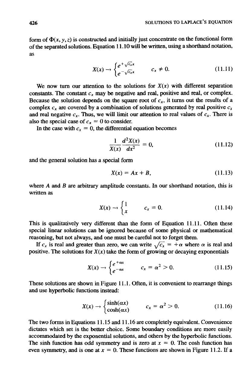
These solutions are shown in Figure 1 1.1. Often, it
is
convenient to rearrange things
and use hyperbolic functions instead:
(11.16)
The two forms in Equations
1
1.15 and
1
1.16 are completely equivalent. Convenience
dictates which set
is
the better choice. Some
boundary
conditions are more easily
accommodated
by
the exponential solutions, and others by
the
hyperbolic functions.
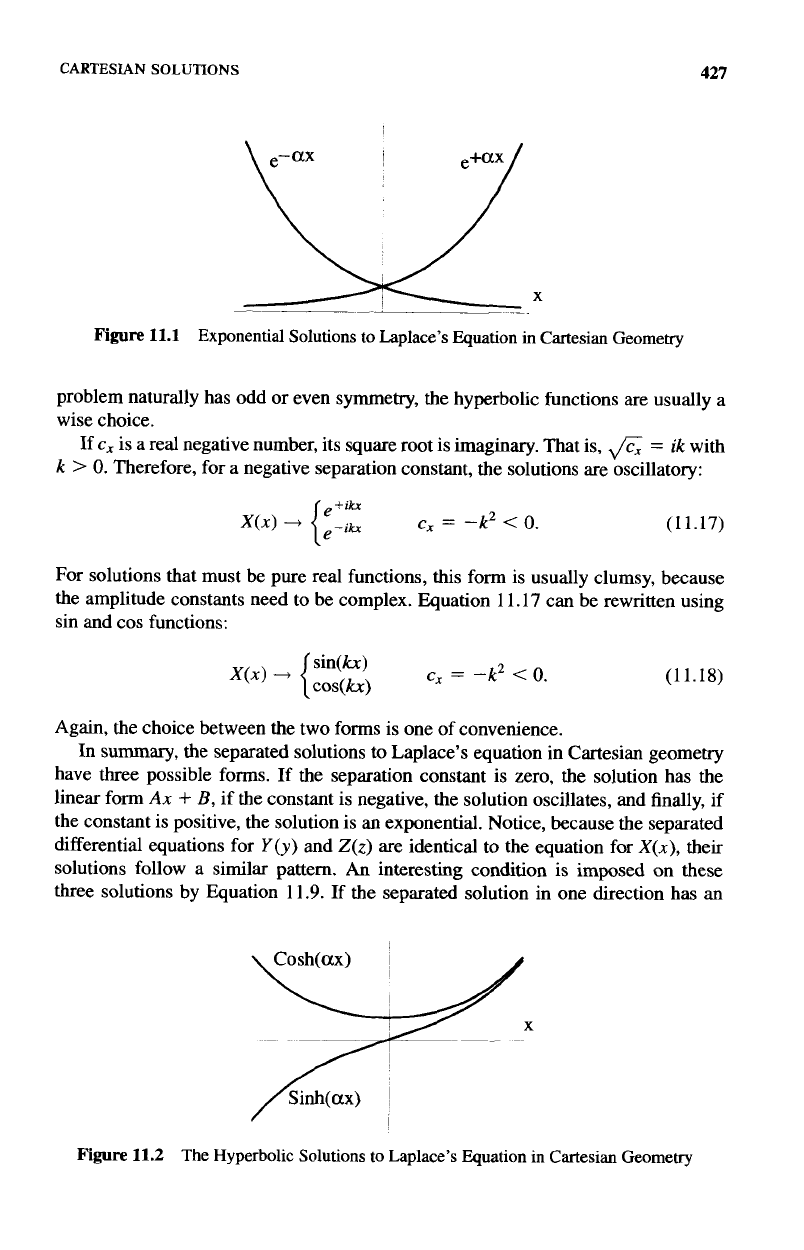
The
sinh
function has odd symmetry and
is
zero at
x
=
0.
The cosh function has
even symmetry, and
is
one at
n
=
0.
These functions are shown
in
Figure 1 1.2.
If
a
CARTESIAN
SOLUTIONS
427
Figure
11.1 Exponential Solutions
to
Laplace’s Equation in Cartesian Geometry
problem naturally has odd or even symmetry, the hyperbolic functions are usually a
wise choice.
=
ik
with
k
>
0.
Therefore, for a negative separation constant, the solutions
are
oscillatory:
If
c,
is a real negative number, its square root is imaginary. That is,
(11.17)
For solutions that must be pure real functions, this form is usually clumsy, because
the amplitude constants need to be complex. Equation
11.17
can be rewritten using
sin and cos functions:
(11.18)
Again, the choice between the two forms is one of convenience.
In
summary,
the separated solutions
to
Laplace’s equation in Cartesian geometry
have three possible forms. If the separation constant is zero, the solution has the
linear form
Ax
+
B,
if the constant is negative, the solution oscillates, and finally, if
the constant is positive, the solution is
an
exponential. Notice, because the separated
differential equations for
Y
(y)
and
Z(z)
are identical to the equation for
X(x),
their
solutions follow a similar pattern.
An
interesting condition is imposed on these
three solutions by Equation 11.9. If the separated solution in one direction has an
Figure
11.2 The Hyperbolic Solutions
to
Laplace’s Equation in Cartesian Geometry
4%
SOLUTIONS
TO
LAPLACE’S
EQUATION
exponential
form,
at least one
of
the other solutions must have an oscillatory form
and vice versa. We will discover that
this
is
a general trait of the separated solutions
in other coordinate systems
as
well.
11.1.2
The
General
Solution
The solution for
+(x,
y,
x)
is
the product
of
the
three
separated solutions, as described
by Equation 1 1.3. The amplitude and separation constants are determined by a set of
boundary conditions. These boundary conditions may allow a particular separation
constant to take on more than one value and, in many cases, an infinite set of
discrete values.
In
such a situation, because Laplace’s equation is linear, the general
solution will be composed
of
a
hear
sum
over the acceptable values of the separation
constants.
Let
the possible nonzero values
of
c,
be indexed by
m.
That
is,
the
mth
allowed
separation constant for
x
is
c,.
Likewise, let
cyn
be the
nth
nonzero separation
constant for the
y
variable. Equation 11.9 implies that
c,
cannot be independently
specified, because
c,
=
-c,
-
cyn.
Using the shorthand notation, we can write the
general solution
as
a
sum
over the two indices
n
and
m:
+
The Special Linear Solutions.
The sum on the
RHS
of
this
equation
is
a shorthand notation for writing all the
combinations of solutions that have nonzero separation constants, each with an un-
determined amplitude constant. For each value of
m
and
n,
there are eight possible
combinations
of
the solution
types.
If
you wanted to expand
this
out,
it
would look
like this:
cc
mn
(11.20)
Many
times the symmetry of the problem
will
eliminate some
of
the terms in the
bracketed sum
of
Quation 11.20, and those particular amplitude constants will be
zero. For
this
reason, it is convenient to use the shorthand notation
of
Equation 1 1.19
and not address the amplitude constants until the symmetry arguments have placed
the general solution in more tractable form.
:ARTESIAN
SOLUTIONS
429
The “special” solutions of Equation 1 1.19 are the ones that fall outside
of
normal
rorm
because one or more of the separation constants is zero. For example, if a
iossible solution has
c,
=
0,
but
cy
=
c
and
cz
=
-c,
there is a special set of linear
jolutions
When
c,
=
cy
=
c,
=
0,
another set of special solutions is
{:
{;
{:
‘
(1
1.21)
(1 1.22)
The general solution will be unique, that is to say all the amplitude and separation
:onstants will be determined,
only
if enough boundary conditions are specified. For
Laplace’s equation this means that the solution will be unique
in
a region if the value
3f
@(x,
y,
z)
or its normal derivative, or a combination of
@(x,
y,
z)
and its normal
derivative is specified over the entire surface enclosing that region. These are referred
to
as
the Neumann or Dirichlet boundary conditions, respectively.
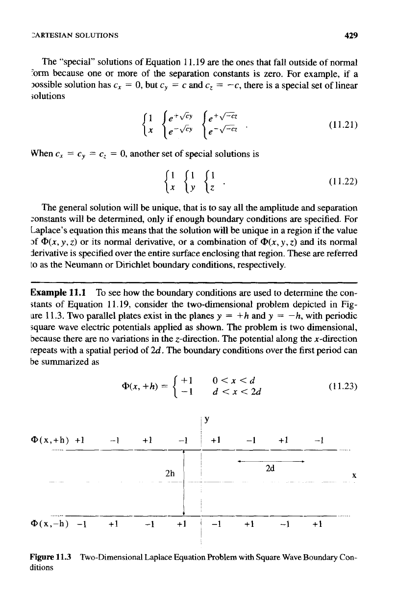
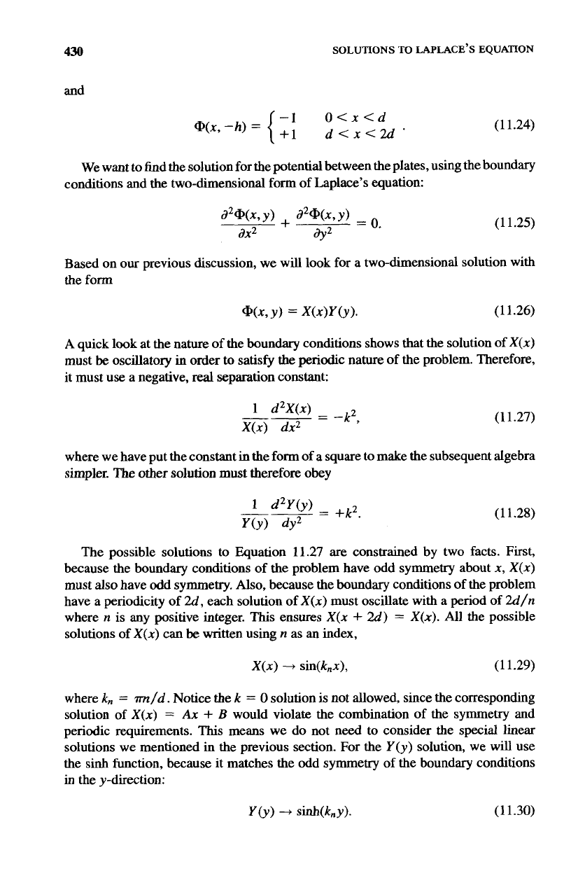
Example
11.1
To
see how the boundary conditions are used to determine the con-
stants of Equation 1 1.19, consider the two-dimensional problem depicted
in
Fig-
ure 11.3.
Two
parallel plates exist in
the
planes
y
=
+h and
y
=
-h,
with periodic
square wave electric potentials applied
as
shown. The problem is two dimensional,
because there are
no
variations in the z-direction. The potential along the x-direction
repeats with a spatial period
of
2d.
The boundary conditions over the first period can
be summarized
as
+1
O<x<d
-1
d<~<2d
@(x,
+h)
=
@(x,+h)
+1
-1
+1 -1
I
+I
-1
+1 -1
(11.23)
2d
@(x,-h)
-1
+I
-1 +1
1
-1
+I
-1
+1
X
Figure
11.3
ditions
Two-Dimensional
Laplace Equation Problem with
Square
Wave
Boundary Con-
430
SOLUTIONS TO LAPLACE’S
EQUATION
and
(11.24)
We want
to
find the solution for the potential between the plates, using the boundary
conditions and the two-dimensional
form
of Laplace’s equation:
(1 1.25)
Based on
our
previous discussion, we will look for a two-dimensional solution with
the form
A
quick look at the nature of the boundary conditions shows that the solution
of
X(x)
must
be
oscillatory in order
to
satisfy the periodic nature of the problem. Therefore,
it must use a negative,
real
separation constant:
(
1 1.27)
where we have put the constant in the
form
of
a square to make the subsequent algebra
simpler. The other solution must therefore obey
(1
1.28)
The possible solutions to muation 11.27 are constrained by two facts. First,
because the boundary conditions of the problem have odd symmetry about
x,
X(x)
must also have odd symmetry.
Also,
because the boundary conditions of the problem
have a periodicity of
2d,
each solution of
X(x)
must oscillate with a period
of
2d/n
where
n
is any positive integer.
This
ensures
X(x
+
2d)
=
X(x).
All
the
possible
solutions of
X(x)
can be written using
n
as an index,
X(x)
--f
sin(k,,x),
(11.29)
where
k,,
=
m/d.
Notice the
k
=
0
solution
is
not allowed, since the corresponding
solution of
X(x)
=
Ax
+
B
would violate the combination of the symmetry and
periodic requirements.
This
means we do not need to consider the special linear
solutions
we
mentioned in the previous section. For the
Y
(y)
solution, we will use
the sinh function, because it matches the odd symmetry of the boundary conditions
in
the y-direction:
CARTESIAN SOLUTIONS
431
The combination of these two solutions generates the general solution for @(x, y),
m
@(x,
Y>
=
C
An
Sin(knX) sinh(kny),
(11.31)
n=1,2,
...
where the amplitude constants
A,
are
finally introduced.
The
A,
coefficients are determined by requiring Equation 1 1.3
1
go to the applied
potential on the boundaries. Since we have already imposed the odd symmetry in
the y-direction, if the expression
in
Equation 11.31 goes to the proper potential at
y
=
+h, it will automatically go to the correct value at
y
=
-h
as well. Thus to
make everything work, the solution must satisfy
a
(
1
1.32)
+1
O<x<d
A,,
sin
(7)
sinh
(F)
=
{
-1 d<x<2d'
n=
1,2,
...
The
LHS
of Equation
11.32
is in the form of a Fourier sine series.
A
particular
coefficient
A,
can be obtained by operating on both sides of
this
equation with
6"
dx sin
(
y)
Every term in the series drops out except the
n
=
m
term, giving the result:
(0
m
even
modd
.
4
Am
=
(
m?r
sinh(m?rh/d)
(1
1.33)
(
1
1.34)
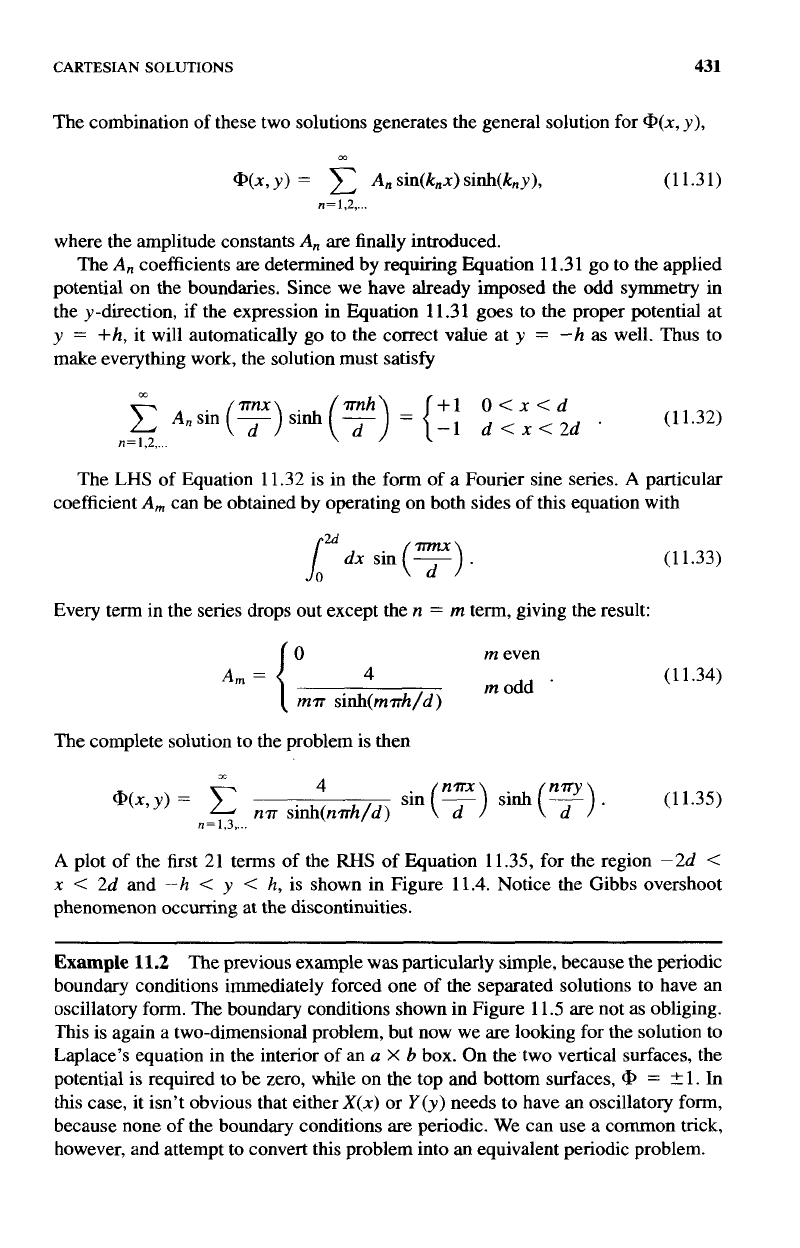
The complete solution
to
the problem is then
cc
4 sin(?) sinh(F). (11.35)
n?r
sinh(n?rh/d)
@(X,Y)
=
c
n=1,3,
...
A
plot of the first 21 terms
of
the
RHS
of Equation 11.35, for the region -2d
<
x
<
2d and
-h
<
y
<
h,
is shown in Figure 11.4. Notice the Gibbs overshoot
phenomenon occurring at the discontinuities.
Example
11.2
The previous example was particularly simple, because the periodic
boundary conditions immediately forced one
of
the separated solutions to have
an
oscillatory form. The boundary conditions shown in Figure 1 1.5 are not as obliging.
This is again a two-dimensional problem, but now we are looking for the solution to
Laplace's equation in the interior
of
an
a
X
b
box. On the two vertical surfaces, the
potential is required to be zero, while
on
the
top
and
bottom surfaces,
CD
=
2
1.
In
this
case, it isn't obvious that either
X(x)
or
Y
(y) needs to have
an
oscillatory form,
because none
of
the boundary conditions are periodic. We can use a common trick,
however, and attempt to convert this problem into
an
equivalent periodic problem.
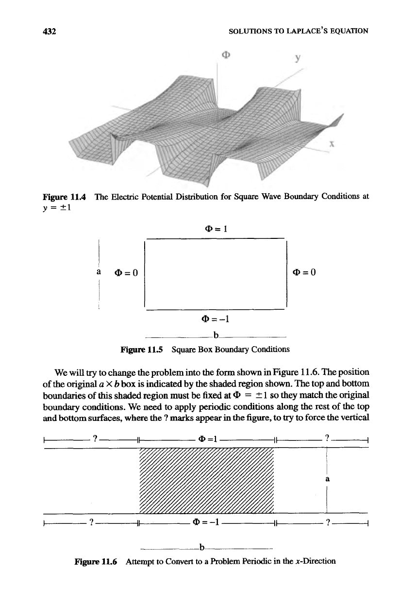
432 SOLUTIONS
TO
LAPLACE'S EQUATION
I
Y
Q,
Figure
11.4
The
Electric
Potential Distribution
for
Square Wave
Boundary
Conditions
at
y
=
?1
a
@=O
i
@=
1
@=O
@=-1
b
Figure
11.5
Square
Box
Boundary
Conditions
We
will
try
to change the problem into the
form
shown in Figure
11.6.
The position
of the original
a
X
b
box
is indicated
by
the
shaded region shown. The top and
bottom
boundaries
of
this
shaded region must be fixed at
=
2
1
so
they match the original
boundary conditions. We need
to
apply periodic conditions along the rest
of
the top
and
bottom
surfaces, where the
?
marks
appear
in
the figure,
to
try
to
force the vertical
-
b
Figure
11.6
Attempt
to
Convert
to
a
Problem Periodic
in
the
x-Direction
EXPANSIONS
WITH
EIGENFUNCTIONS
433
@
=1
@=-I
@
=1
@=-1
@
=1
a
/
@=-1
@
=I
@=-1
@
=1
@=-1
--bp
~-
Figure
11.7
Conversion
to
a
Periodic
Problem
in
the
x-Direction
sides
of
the shaded region to have
@
=
0.
Looking back on the previous example,
it is pretty easy to see that these requirements are met with the potential distribution
shown in Figure 1
1.7.
The solution inside the box is therefore identical to the solution
to the previous example with the x-periodicity equal to
26.
The only difference is, of
course, that this solution is only valid inside the region of the original
a
X
b
box of
Figure 11.5.
We successfully made this problem periodic
in
the x-direction. Could we have
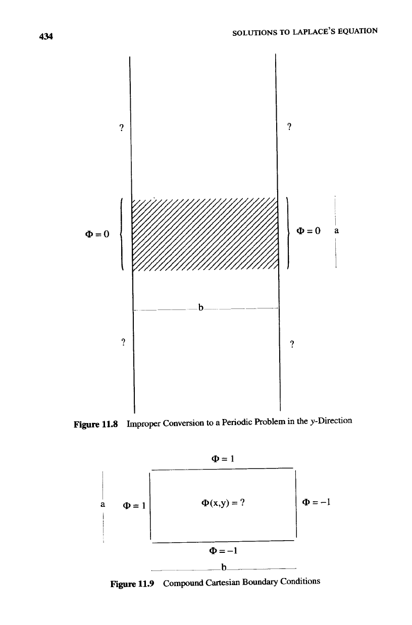
done the same thing in the y-direction? Figure 11.8 shows what this would look like.
Again, we need to apply periodic potentials to the areas where the
?
marks occur in
the figure,
to
try
to force the horizontal sides of the shaded region to have
@
=
2
1.
It’s pretty obvious this cannot work. In
this
case, the x-direction must
be
chosen as
the periodic one.
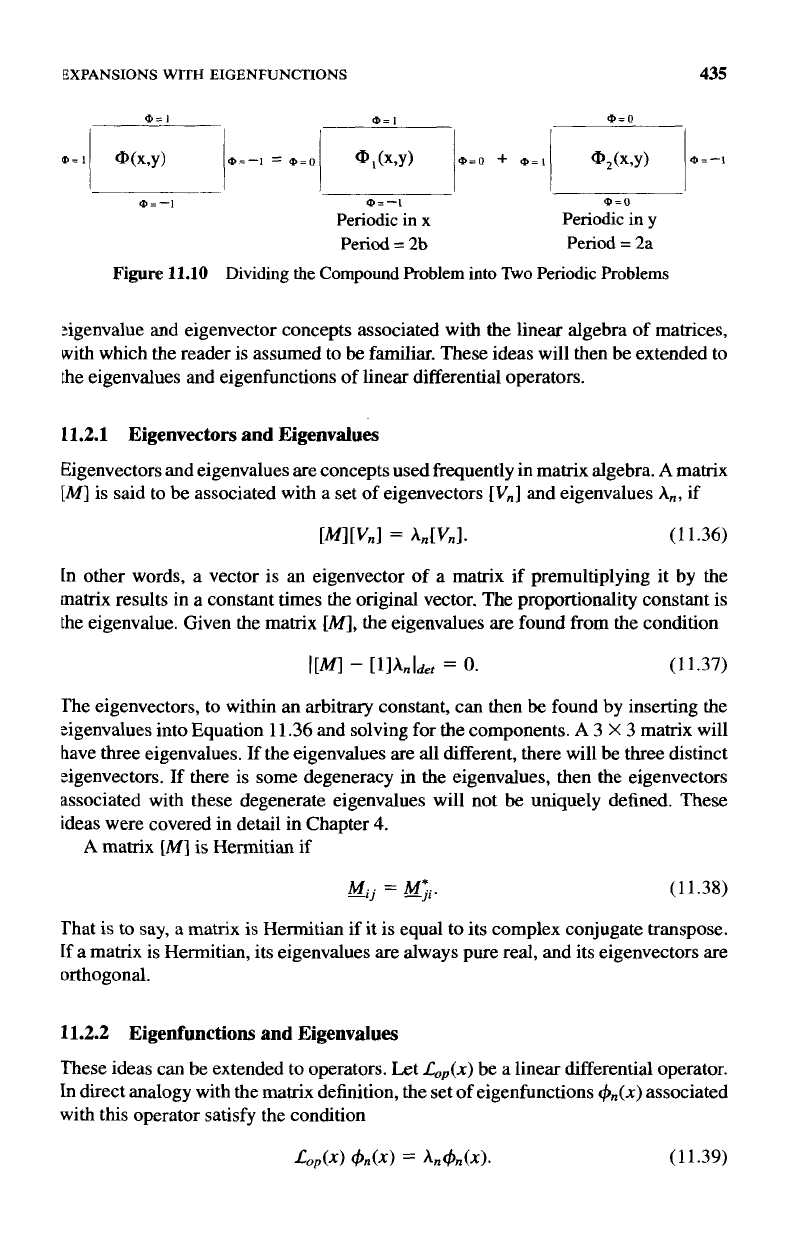
An interesting twist is added
to
this problem if we modify the boundary conditions,
as
shown in Figure
1
1.9. In a case llke this, you will find it is impossible to simply
make either the
x-
or
y-direction periodic. Instead, the problem must be broken up
into two parts,
as
shown in Figure 11.10, Because Laplace’s Equation
is
linear, the
solution can be written as the
sum
of two solutions,
@I
(x,
y) and
@*(x,
y),
which
each satisfy modified boundary conditions shown
for
the two boxes on the right. The
function
@~(x,
y)
satisfies Laplace’s equation and has boundary conditions which are
amenable
to
periodic extension in the x-direction. The function
@(x,
y) also satisfies
Laplace’s equation, but with conditions which can be extended in the y-direction.
The combination
Q1(x,
y)
+
Q2(x,
y)
=
@(x,
y) satisfies Laplace’s equation inside
the box and satisfies the original boundary conditions of Figure 1
1.9.
11.2
EXPANSIONS WITH ELGENFUNCTIONS
Before looking at solutions to Laplace’s equation in other coordinate systems, we need
to establish some general techniques for expanding functions with linear summations
of
orthogonal functions. In the Cartesian problems we have discussed
so
far, we found
that we could evaluate the individual amplitude constants in the general solution by
using Fourier series type orthogonality conditions.
This
worked because the terms in
our sums
of
the general solution contained sine and cosine functions. In this section,
we will generalize this technique for other problems. We will begin by reviewing the
434
,
@=O
I
?
SOLUTIONS
TO
LAPLACE’S
EQUATION
a,=O
?
Figure
11.8
Improper
Conversion
to
a
Periodic Problem in
the
y-Direction
@=1
a
a,=l
I
I
@(x,y)
=
?
@=-I
a,=-1
b
Figure
11.9
Compound Cartesian Boundary Conditions
EXPANSIONS
WITH EIGENFUNCTIONS
435
O=
I
8=
I
8=
1
O=O
@=-I
@=-I
,#=O
Periodic in
x
Period
=
2b
Periodic
in
y
Period
=
2a
Figure
11.10
Dividing the
Compound
Problem
into
Two
Periodic Problems
:igenvalue and eigenvector concepts associated with the linear algebra of matrices,
with which the reader is assumed to
be
familiar. These ideas will then be extended to
Lhe eigenvalues and eigenfunctions of linear differential operators.
11.2.1 Eigenvectors and Eigenvalues
Eigenvectors and eigenvalues are concepts used frequently in matrix algebra.
A
matrix
[MI
is said to be associated with a set of eigenvectors
[
Vn]
and eigenvalues
A,,
if
[W[Vnl
=
An[VnI-
(1
1.36)
[n other words, a vector is an eigenvector of a matrix if premultiplying it by the
matrix results in a constant times the original vector. The proportionality constant
is
the eigenvalue. Given the matrix
[MI,
the eigenvalues are found from the condition
I[Ml
-
[lIAnIdet
=
0.
(11.37)
The eigenvectors, to within an arbitrary constant, can then
be
found by inserting the
zigenvalues into Equation
11.36
and solving for the components.
A
3
X
3
matrix will
have three eigenvalues. If the eigenvalues are all different, there will be
three
distinct
eigenvectors. If there is some degeneracy
in
the eigenvalues, then the eigenvectors
associated with these degenerate eigenvalues will not
be
uniquely defined. These
ideas were covered in detail in Chapter
4.
A
matrix
[MI
is Hermitian
if
M..
=
M*..
(11.38)
That is to say, a matrix is Hermitian if it is equal
to
its complex conjugate transpose.
If
a matrix is Hermitian, its eigenvalues are always pure real, and its eigenvectors are
orthogonal.
dJ
--J
11.2.2 Eigenfunctions and Eigenvalues
These ideas can be extended to operators. Let
L,,(x>
be a linear differential operator.
In direct analogy with the matrix definition, the set of eigenfunctions
&(x)
associated
with this operator satisfy the condition
Lop(x>
&(X)
=
An4n(x).
(1
1.39)