Mann U. Principles of Chemical Reactor Analysis and Design: New Tools for Industrial Chemical Reactor Operations

Подождите немного. Документ загружается.

We select the forward reaction as the independent reaction and the reverse reaction

as the dependent rea ction. Hence, the inde x of the independent reaction is m ¼ 1,

the index of the dependent reaction is k ¼ 2. Since Reaction 2 is the reverse of

Reaction 1, a

¼ 21. The stoichiometric coefﬁcients of the independent r eaction ar e

¼1 s

¼ 1 D

¼ 0

Using Eq. 6.1.1, and selecting the initial sta te as the refer ence s ta te, for a cons tant-

volume reaction

¼ (r

 r

)



(6:3:1)

Using Eq. 6.1.12 to expr ess the species concentr a tions, the two reaction rates are

¼ k

[ y

(0)  Z

]

¼ k

[ y

(0) þ Z

]

We deﬁne the characteristic reaction time on the basis of Reaction 1:

Substituting these rela tions into Eq. 6.3.1, the design equa tion r educes to

¼ [ y

(0)  Z

] 



[ y

(0) þ Z

](6:3:2)

To simplify the design equa tion, we rearr ange Eq. 6.3.2 and notice that, a t equilibrium,

(dZ

/dt ¼ 0),

(0)  (k

(0)

1 þ (k

)

(6:3:3)

where Z

is the dimensionless extent at equilibrium. Using Eq. 6.3.3, the design

equation becomes

þ k



 Z

)(6:3:4)

Separating the variables and integrating, we obtain

Z(t) ¼ Z

1  exp 

þ k



(6:3:5)

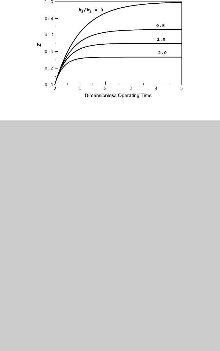
Figure 6.8 showsthe reaction operating curve for different values of k

. Note that the

design equation for batch reactors with single reversible reactions has two parameters

and k

), whereas the design equation for reactors with an irreversible reaction has

only one parameter. Also note that for an irreversible rea ction, k

¼ 0, and, from

Eq. 6.3.3, Z

¼ y

(0).

200 IDEAL BATCH REACTOR

Example 6.8 The reversible gas-phase chemical reaction



takes place in an isothermal batch reactor. The forward reaction is ﬁrst order, and

the backward reaction is second order. We charge 100 mol of reactant A into the

reactor that operates at 1208C. The initial pressure is 2 atm. At the operating con-

ditions (1208C), k

¼ 0.1 min

and k

¼ 0.322 L mol

min

a. Derive the design equation and plot the reaction curve for a constant-volume

batch reactor.

b. Determine the equilibrium composition at 1208C in a constant-volume

reactor.

c. Determine the operating time to obtain 90% of the equilibrium conversion?

d. Derive the design equation and plot the reaction curve for an isobaric, vari-

able-volume batch reactor.

e. Determine the equilibrium composition at 1208C in an isobaric variable-

volume reactor.

f. What is the operating time to obtain 90% of the equilibrium conversion?

Solution We write the reversible reaction as two separate reactions:

Reaction 1: A ! 2B

Reaction 1: 2B ! A

whose stoichiometric coefﬁcients are

¼1 s

¼ 2 D

¼ 1

¼ 1 s

¼2 D

¼1

Figure 6.8 Reaction operating curves for single reversible reaction.

6.3 ISOTHERMAL OPERATIONS WITH MULTIPLE REACTIONS 201

We have here one independent reaction, and select Reaction 1 as the independent

reaction; hence, the reaction indices are m ¼ 1 and k ¼ 2, and, for a reversible

reaction, a

¼ 2 1. We select the initial state as the reference state, and the

reference concentration is

2 atm

(82:06 10

3

L atm=mol K)(393 K)

¼ 0:062 mol=L (a)

Since only reactant A is charged to the reactor, y

(0) ¼ 1 and y

(0) ¼ 0.

a. We use Eq. 6.1.1; for a constant-volume batch reactor the design equation is

¼ (r

 r

)



(b)

We deﬁne the characteristic reaction time on the basis of reaction 1:

¼ 10 min (c)

Equation 6.1.12 expresses the species concentrations; the reaction rates of the

two reactions are

¼ k

(1  Z

) r

¼ k

(2Z

)

Substituting the rates and (c) into (b), the design equation reduces to

¼ 1  Z





(d)

Once we solve the design equation, we use Eq. 2.7.4 to obtain the species

curves:

(t)

tot

)

¼ 1  Z

(t) (e)

(t)

tot

)

¼ 2Z

(t)(f)

Using Eq. 2.7.6

tot

(t)

tot

)

¼ 1 þ Z

(t) (g)

For the given data, k

¼ 0.2, and we solve (d) subject to the initial

condition that Z

(0) ¼ 0. Figure E6.8.1 shows the reaction operating curve

202 IDEAL BATCH REACTOR

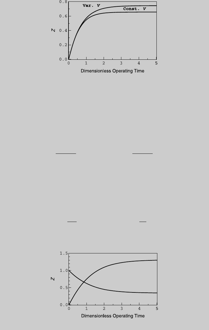
and compares it to the reaction curve obtained on a variable-volume batch

reactor. Using (e) and (f), we determine the species curves shown in

Figure E6.8.2.

b. At equilibrium, dZ

/dt ¼ 0, and, the equilibrium extent is Z

1eq

¼ 0:6563.

Using (e), (f), and (g), the species molar fractions at equilibrium are

1  Z

1 þ Z

¼ 0:2075 y

1 þ Z

¼ 0:7925

c. A level of 90% equilibrium conversion corresponds to Z ¼ 0.5907, and, from

the reaction curve, it is reached at t ¼ 1.26. Using (c), the operating time is

t ¼ t

t ¼ 12:6 min

d. For an isobaric, variable-volume batch reactor, the design equation Eq. 6.1.1 is

¼ (r

 r

)(1 þ D

)



(h)

Figure E6.8.1 Reaction curves.

Figure E6.8.2 Species curves.

6.3 ISOTHERMAL OPERATIONS WITH MULTIPLE REACTIONS 203

Using Eq. 6.1.16 to express the species concentrations, the reaction rates are

¼ k

1  Z

1 þ Z



¼ k

1 þ Z



(i)

Substituting the rates and (c) into (h), the design equation becomes

¼ 1  Z





1 þ Z

(j)

We solve ( j) subject to the initial condition that Z

(0) ¼ 0. The reaction curve

is shown in Figure E6.8.1.

e. At equilibrium, dZ

/dt ¼ 0, and, from ( j), the equilibrium extent is

¼ 0.7455. Using (e), (f), and (g), the species molar fractions at equili-

brium are

1  Z

1 þ Z

¼ 0:1458 y

2  Z

1 þ Z

¼ 0:8542

f. A level of 90% equilibrium conversion corresponds to Z ¼ 0.671 and, from

the operating curve, it is reached at t ¼ 1.56; using (c), the operating time is

15.6 min.

Next, we consider series (consecutive) chemical reactions. These are reactions

where the product of one reaction reacts to form undesirable species. In such

cases, it is important to consider the amount of desirable and undesirable products

formed in addition to the conversion of the reactant. In many instances, the yield of

the desirable product provides a measure of the reactor performance.

Example 6.9 A valuable product B is produced in a batch reactor where the

following liquid-phase reactions take place:

Reaction 1: A ! 2B

Reaction 2: B ! C þ D

Each chemical reaction is ﬁrst order. The reactor is charged with 200 L of an

organic solution with a concentration of 4 mol A/L. The reactor is operated at

1208C. At the reactor temperature, k

¼ 0.05 min

and k

¼ 0.025 min

a. Derive the design equations and plot the reaction and species curves.

b. Derive an expression for the yield of product B, and plot it as a function of the

operating time.

204 IDEAL BATCH REACTOR

c. Determine the operating time when the production of product B is

maximized.

d. Determine the conversion of reactant A and the yield and selectivity of

product B at optimal operating time.

Solution This is an example of series (sequential) chemical reactions. The

stoichiometric coefﬁcients of the chemical reactions are

¼1 s

¼ 2 s

¼ 0 s

¼ 0 D

¼ 1

¼ 0 s

¼1 s

¼ 1 s

¼ 1 D

¼ 1

Since each reaction has a species that does not participate in the other, the two

reactions are independent, and there is no dependent reaction.

a. We write Eq. 6.1.1 for each independent reaction:

¼ r



(a)

¼ r



(b)

We select the initial state as the reference sate; hence, C

¼ C

(0), and

tot

)

¼ V

(0)C

¼ 800 mol

Since only reactant A is charged into the reactor, y

(0) ¼ 1, and

(0) ¼ y

(0) ¼ 0. We use Eq. 6.1.12 to express the species concen-

trations, and the rates of the two reactions are

¼ k

(1  Z

) (c)

¼ k

(2Z

 Z

) (d)

We select reaction 1, the desirable reaction, to deﬁne the characteristic reac-

tion time

¼ 20 min (e)

Substituting (c), (d), and (e) into (a) and (b), the two design equations reduce to

¼ 1  Z

(f)



(2Z

 Z

) (g)

6.3 ISOTHERMAL OPERATIONS WITH MULTIPLE REACTIONS 205

After we solve the design equa tions, we use Eq. 2.7.4, to determine the species

curves,

tot

)

¼ 1  Z

(h)

tot

)

¼ 2Z

 Z

(i)

tot

)

tot

)

¼ Z

(j)

In this case, the two design equations are not coupled, and we can obtain

analytical solutions. We solve (f) subject to the initial condition that

(0) ¼ 0, and obtain

(t) ¼ 1  e

t

(k)

W e substitute (k) into (g), and the second design equa tion reduces to



¼ 2



(1  e

t

) (l)

This is a ﬁrst-order linear differ ential equation tha t can be solved analytically

by using an integra ting factor. W e solv e (l) subject to the initial condition

that Z

(0) ¼ 0, and obtain

(t) ¼ 21

 k



(k

 k



t



(m)

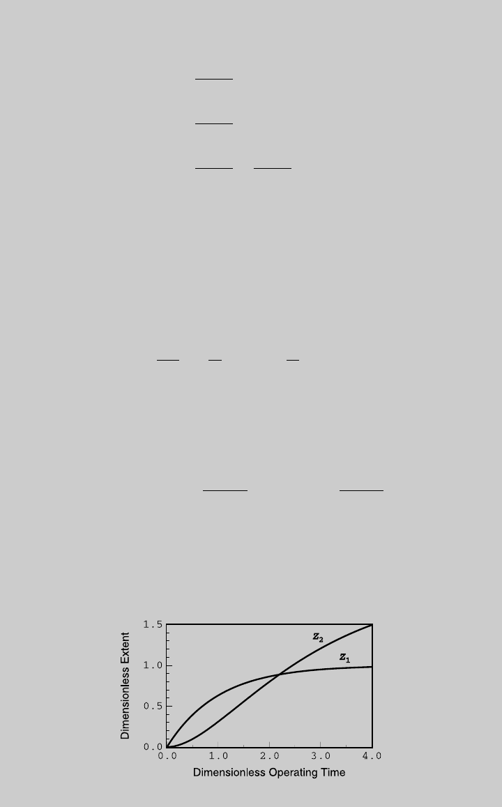
For the given data, k

¼ 0:5, we plot Z

(t)andZ

(t) in Figure E6.9.1. Once

we have Z

(t)andZ

(t), we use (h) through ( j) to plot the species curves,

shown in Figure E6.9.2.

Figure E6.9.1 Reaction curves.

206 IDEAL BATCH REACTOR

b. The desirable chemical reaction is Reaction 1, and using Eq. 2.6.12, the yield

of product B is

(t) ¼



(t) N

(0)



and, using (i),

(t) ¼

[2Z

(t)  Z

(t)] ¼ Z

(t)  0:5Z

(t) (n)

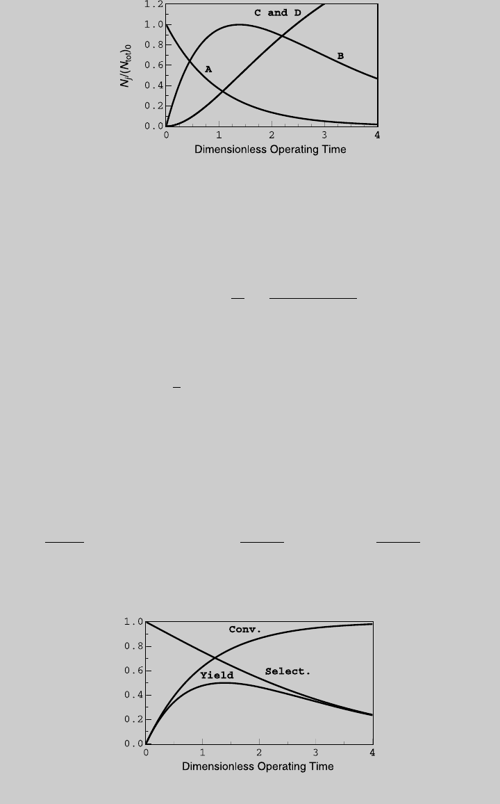
Figure E6.9.3 shows the yield curve.

c. To determine the optimal operating time, we use either the curve of product B

or the analytical solutions. From the graph, maximum N

is reached at

t ¼ 1.39. Alternatively, using (i), (k), and (m),

(t)

tot

(0)

¼ 2(1  e

t

)  21

 k



(k

 k



t



(o)

Figure E6.9.2 Species curves.

Figure E6.9.3 Yield and selectivity.

6.3 ISOTHERMAL OPERATIONS WITH MULTIPLE REACTIONS 207

To determine the maximum, we take the derivative of (o) with respect to t

and equate it to zero

max

 k



 k



(q)

For k

¼ 0.5, t

max

¼ 1.39. Using (e), the optimal operating time is

t ¼ tt

¼ 27:6 min

d. For t ¼ 1.39, the solutions of (l) and (n) are Z

¼ 0.751 and Z

¼ 0.502.

Using (i) and (j), the species amounts are: N

¼ 199.2 mol. Using (h), the

conversion of reactant A is

(

) ¼

(0)  N

(

)

(0)

¼ 0:751

Using (n), the yield of product B is 0.5. To calculate the selectivity of product

B, we use Eq. 2.6.17, (h), and (i),

(

) ¼

1



(

)  Z

(

)

(

)

¼ 0:666

The selectivity curve is shown in Figure E6.9.3.

Next, we consider parallel chemical reactions. These are reactions in which a

reactant of the desirable reaction also reacts in another reaction to form undesirable

species. In such cases, it is important to consider not only the conversion of the

reactant but also the amount of desirable and undesirable products formed. The

yield of the desirable product provides a measure of the reactor performance.

Example 6.10 The catalytic oxidation of propylene on bismuth molybdate to

produce acrolein is investigated in a constant-volume batch reactor. The follow-

ing chemical reactions take place in the reactor:

Reaction 1: C

þ O

! C

O þ H

Reaction 2: C

O þ 3:5O

! 3O

þ 2H

Reaction 3: C

þ 4:5O

! 3CO

þ 3H

208 IDEAL BATCH REACTOR

The rate of each reaction is second order (ﬁrst order with respect to each reac-

tant), and the reaction rate constants at 4608Carek

¼ 0.5 L mol

, k

¼ 0.25, k

¼ 0.10. A gas mixture consisting of 60% propylene and 40%

oxygen is charged into a 4-L isothermal reactor operated at 4608C. The initial

pressure is 1.2 atm.

a. Derive the design equations, and plot the reaction and species operating

curves.

b. Determine the operating time needed for 75% conversion of oxygen.

c. Determine the reactor composition at 75% conversion of oxygen.

Solution The reactor design formulation of these chemical reactions was dis-

cussed in Example 4.2. Recall that there are two independent reactions and one

dependent reaction, and, following the heuristic rule, we select Reactions 1 and 2

as a set of independent reactions; hence, m ¼ 1, 2, and k ¼ 3. The stoichiometric

coefﬁcients of the independent reactions are

)

¼1(s

)

¼1(s

)

¼1(s

)

¼1(s

)

¼0 D

¼0

)

¼0(s

)

¼3:5(s

)

¼1(s

)

¼2(s

)

¼3 D

¼0:5

Recall from Example 4.2 that the multipliers a

’s of the dependent reaction

(Reaction 3) and the two independent reactions (Reactions 1 and 2) are

¼ 1 and a

¼ 1. We select the initial state as the reference state; hence,

¼0:02mol=L (a)

tot

)

¼V

(0)C

¼0:08mol

The initial composition is

(0)¼0:6 y

(0)¼0:4 y

(0)¼y

(0)¼0

a. We write Eq. 6.1.1 with V

(t) ¼ V

(0) ¼ V

for each the independent

reaction,

¼ (r

þ r

)



(b)

¼ (r

þ r

)



(c)

6.3 ISOTHERMAL OPERATIONS WITH MULTIPLE REACTIONS 209