Mann U. Principles of Chemical Reactor Analysis and Design: New Tools for Industrial Chemical Reactor Operations
Подождите немного. Документ загружается.

where V
inj
is the total volume injected during the operation. The concentration of
the reference state, C
0
, is defined by
C
0
;
(N
tot
)
0
V
R
0
(9:1:10)
The dimensionless time is defined by
t ;
t
t
cr
(9:1:11)
where t
cr
is the characteristic reaction time, defined in Section 3.5 (Eq. 3.5.1).
Differentiating Eq. 9.1.7 and Eq. 9.1.11,
dX
m
¼ (N
tot
)
0
dZ
m
dt ¼ t
cr
dt
and substituting these into Eq. 9.1.2, the dimensionless design equation for semi-
batch reactor is
dZ
m
dt
¼ r
m
þ
X
n
D
k¼1
a
km
r
k
!
V
R
(t)
V
R
0
t
cr
C
0
0 t t
op
(9:1:12)
where V
R
(t) is given by Eq. 9.1.5 with t ¼ t
cr
t. Equation 9.1.12 is the general
design equation of liquid-phase semibatch reactors with any given injection rate,
written for the mth-independent reaction. To describe the reactor operation, we
have to write the design equation for each independent chemical reaction. Note
that Eq. 9.1.12 is valid only for 0 t t
op
, where t
op
is the dimensionless oper-
ating time defined by
t
op
;
t
op
t
cr
(9:1:13)
To solve the design equations, we should express the rates of all the chemical
reactions (r
m
’s and r
k
’s) in terms of the extents of the independent reactions. The
concentration of species j at time t is
C
j
(t) ;
N
j
(t)
V
R
(t)
(9:1:14)
Using Eq. 2.3.3, the molar content of species j at time t is
N
j
(t) ¼ N
j
(0) þ
ð
t
0
v
inj
(x)(C
j
)
inj
dx þ
X
n
I
m
(s
j
)
m
X
m
(t)(9:1:15)
where the first term on the right, N
j
(0), indicates the number of moles of species
j charged to the reactor initially, the second term indicates the moles of species j
380 OTHER REACTOR CONFIGURATIONS

injected during time t, and the third term indicates the mole of species j formed by
chemical reactions. Substituting Eq. 9.1.15 into Eq. 9.1.14,
C
j
(t) ¼
N
j
(0) þ
Ð
t
0
v
inj
(x)(C
j
)
inj
dx þ
P
n
I
m
(s
j
)
m
X
m
(t)
V
R
(0) þ
Ð
t
0
v
inj
(x) dx
(9:1:16)
Using Eq. 9.1.7 and Eq. 9.1.11, the concentration of species j at dimensionless time
t is
C
j
(t) ¼ C
0
[1=(N
tot
)
0
] N
j
(0) þ
Ð
t
cr
t
0
v
inj
(x)(C
j
)
inj
dx
þ
P
n
I
m
(s
j
)
m
Z
m
(t)
[1=V
R
0
] V
R
(0) þ
Ð
t
cr
t
0
v
inj
(x) dx
(9:1:17)
For a species that is not charged initially into the reactor, N
j
(0) ¼ 0, and for a
species that is not injected continuously, (C
j
)
inj
¼ 0.
When the injection rate is uniform, v
inj
(t) ¼ (v
0
)
inj
, Eq. 9.1.5 becomes
V
R
(t) ¼ V
R
(0) þ (V
0
)
inj
t (9:1:18)
and using Eq. 9.1.9, the injection rate is
(v
0
)
inj
¼
V
inj
t
op
¼
V
R
0
V
R
(0)
t
op
(9:1:19)
where V
inj
is the total injected volume. Substituting Eq. 9.1.18 and Eq. 9.1.19 into
Eq. 9.1.12, the design equation of semibatch reactors with a uniform injection
rate is
dZ
m
dt
¼ r
m
þ
X
n
D
k
a
km
r
k
!
V
R
(0)
V
R
0
þ
V
inj
V
R
0
t
t
op
t
cr
C
0
0 t t
op
(9:1:20)
and Eq. 9.1.17 reduces to
C
j
(t) ¼ C
0
N
j
(0)
(N
tot
)
0
þ
(N
j
)
inj
(N
tot
)
0
t
t
op
þ
X
n
I
m
(s
j
)
m
Z
m
(t)
V
R
(0)
V
R
0
þ
V
inj
V
R
0
!
t
t
op
(9:1:21)
9.1 SEMIBATCH REACTORS 381

For constant volume, gas-phase semibatch reactors, V
R
(t) ¼ V
R
(0) ¼ V
R
0
, and
the design equation (Eq. 9.1.2) reduces to
dX
m
dt
¼ r
m
þ
X
n
D
k¼1
a
km
r
k
!
V
R
0
(9:1:22)
Substituting Eq. 9.1.7 and Eq. 9.1.11 into Eq. 9.1.22, the dimensionless design
equation is
dZ
m
dt
¼ r
m
þ
X
n
D
k¼1
a
km
r
k
!
t
cr
C
0
(9:1:23)
Using Eq. 9.1.17, the concentration of species j at time t is
C
j
(t) ¼ C
0
N
j
(0)
(N
tot
)
0
þ
1
(N
tot
)
0
ð
t
cr
t
0
v
inj
(x)(C
j
)
inj
dx þ
X
n
I
m
(s
j
)
m
Z
m
(t)
2
4
3
5
(9:1:24)
For uniform injection rate, v
inj
(t) ¼ (v
0
)
inj
, and using Eq. 9.1.19, the concentration
of species j is
C
j
(t) ¼ C
0
N
j
(0)
(N
tot
)
0
þ
(N
j
)
inj
(N
tot
)
0
t
t
op
þ
X
n
I
m
(s
j
)
m
Z
m
(t)
$%
(9:1:25)
To express the temperature changes, we write the energy balance equation. For
semibatch reactors, the expansion work is usually negligible, and assuming isobaric
operation, the energy balance equation is
DH(t) ¼ H(t) H(0) ¼ Q(t) þ
ð
t
0
(
_
m
inj
h
inj
) dt W
sh
(t)(9: 1:26)
where (m
˙
inj
h
inj
) is the rate enthalpy added to the reactor by the injection stream.
Assuming no phase change, the change in the enthalpy of the reacting fluid is
H(t) H(0) ¼ M(t)
c
p
[T(t) T
0
] M(0)
c
p
[T(0) T
0
]
þ
X
n
I
m
DH
R
m
(T
0
)X
m
(t)(9:1:27)
382 OTHER REACTOR CONFIGURATIONS

Differentiating Eq. 9.1.26 and Eq. 9.1.27 with respect t o time and noting that
dM/dt ¼ m
˙
inj
,
dH
dt
¼
_
Q þ
_
m
inj
h
inj
_
W
sh
dH
dt
¼ [M(t)
c
p
]
dT
dt
þ
_
m
inj
c
p
[T(t) T
0
] þ
X
n
I
m
DH
R
m
(T
0
)
dX
m
dt
(9:1:28)
where [M(t)
c
p
] is the heat capacity of the reacting fluid at time t. The rate heat is
transferred to the reactor, Q
˙
, and is expressed by
_
Q ¼ U
S
V
V
R
(t)(T
F
T)(9:1:29)
Combining Eqs. 9.1.27, 9.1.28, and 9.1.29, and noting that from overall
material balance
dM
dt
¼
_
m
inj
for reactors with negligible shaft work,
dT
dt
¼
1
M(t)
c
p
"
U
S
V
V
R
(t)(T
F
T)þ
_
m
inj
c
p
[T T
0
]
_
m
inj
h
inj
X
n
I
m
DH
R
m
(T
0
)
dX
m
dt
#
(9:1:30)
Equation 9.1.30 describes the change in the reactor temperature.
To reduce Eq. 9.1.30 to dimensionless form, we relate the heat capacity of the
reacting fluid to that of the reference state by defining a correction factor
M(t)
c
p
; CF(N
tot
)
0
^
c
p
0
(9:1:31)
where CF is the correction factor of the heat capacity at time t, and define the
dimensionless temperature by
u ;
T
T
0
(9:1:32)
where T
0
is the temperature of the reference state.
For liquid-phase semibatch reactors, the enthalpy of the injected stream is
_
m
inj
h
inj
¼
_
m
inj
c
p
inj
(T
inj
T
0
)(9:1:33)
9.1 SEMIBATCH REACTORS 383

where
c
p
inj
is the specific mass-based heat capacity of the injection stream. The total
mass of reacting fluid added to the reactor during the entire operation, M
tot
,is
M
tot
; V
R
(0)r þ
ð
t
op
0
v
inj
(x)r
inj
dx (9:1:34)
The specific molar-based heat capacity,
^
c
p
0
, of the reference state is defined by
^
c
p
0
;
M
tot
c
p
(N
tot
)
0
(9:1:35)
where (N
tot
)
0
is defined by Eq. 9.1.8. For liquid-phase reactions, assuming constant
density and constant specific heat capacity, the correction factor of the heat
capacity is
CF ¼
M(t)
c
p
M
tot
c
p
¼
V
R
(t)
V
R
0
(9:1:36)
where V
R
(t) is given by Eq. 9.1.5 with t ¼ t
cr
t. When there is no change in phase,
_
m
inj
h
inj
¼
_
m
inj
c
p
bT
inj
T
0
c
Using Eqs. 9.1.7, 9.1.10, 9.1.11, 9.1.32, and 9.1.36, Eq. 9.1.30 reduces to
du
dt
¼
1
CF
HTN
V
R
V
R
0
(u
F
u) þ
_
m
inj
t
cr
c
p
(N
tot
)
0
^
c
p
0
(u
inj
u)
X
n
I
m
DHR
m
dZ
m
dt
"#
(9:1:37)
where HTN is the heat-transfer number, defined by Eq. 5.2.22:
HTN ;
Ut
cr
C
0
^
c
p
0
S
V
and DHR
m
is the dimensionless heat of reaction of the mth-independent reaction,
defined by Eq. 5.2.23,
DHR
m
;
DH
R
m
(T
0
)
T
0
^
c
p
0
When the injection rate is uniform,
_
m
inj
¼
M
inj
t
op
384 OTHER REACTOR CONFIGURATIONS

Eq. 9.1.37 reduces to
du
dt
¼
1
CF
HTN
V
R
V
R
0
(u
F
u) þ
1
t
op
V
inj
V
R
0
(u
inj
u)
X
n
I
m
DHR
m
dZ
m
dt
"#
(9:1:38)
Eq. 9.1.36 reduces to
CF ¼
V
R
(0)
V
R
0
þ
V
inj
V
R
0
t
t
op
(9:1:39)
For gas-phase reactions, the heat capacity of the reacting fluid may vary with
both the composition and temperature, and specific molar heat capacities are
used. The rate enthalpy added by the injection stream is
_
m
in
h
in
¼
X
J
j
(F
j
)
inj
^
c
p
j
(T
inj
)
!
(T
inj
T
0
)(9:1:40)
where (F
j
)
inj
is the injection molar flow rate of species j. The heat capacity of the
reference state is
(N
tot
)
0
^
c
p
0
;
X
J
J
[N
j
(0) þ (N
j
)
inj
]
^
c
p
j
(T
0
)(9:1:41)
and the specific molar-based heat capacity of the reference state is
^
c
p
0
;
1
(N
tot
)
0
X
J
j
[N
j
(0) þ (N
j
)
inj
]
^
c
p
j
(T
0
)(9:1:42)
For gas-phase reactions, the heat capacity of the reacting fluid is written in terms of
the species molar contents:
M
c
p
;
X
J
j
N
j
^
c
p
j
(T)(9:1:43)
Differentiating with respect to time
dM
dt
c
p
¼
X
J
j
dN
j
dt
^
c
p
j
(T)(9:1:44)
From material balance over species j,
dN
j
dt
¼ (F
j
)
inj
þ
X
n
I
m
(s
j
)
m
dX
m
dt
(9:1:45)
9.1 SEMIBATCH REACTORS 385

Substituting Eqs. 9.1.31, 9.1.40, 9.1.43, 9.1.44, and 9.1.45 into Eq. 9.1.30 and then
reducing the energy balance equation to dimensionless form, we obtain
du
dt
¼
1
CF(Z
m
, u)
HTN(u
F
u) þ
t
cr
P
J
j
(F
j
)
inj
^
c
p
j
(u
inj
)
(N
tot
)
0
^
c
p
0
(u
inj
1)
2
6
6
6
4
3
7
7
7
5
1
CF(Z
m
, u)
X
J
j
X
n
I
m
(s
j
)
m
dZ
m
dt
!
^
c
p
j
(u)[u 1] þ
X
n
I
m
DHR
m
dZ
m
dt
"#
(9:1:46)
Equation 9.1.46 is the dimensionless energy balance equation for gas-phase,
constant-volume semibatch reactors. The correction factor of the heat capacity is
CF(Z
m
, u) ¼
X
J
j
N
j
(0)
(N
tot
)
0
þ
1
(N
tot
)
0
ð
t
cr
t
0
(F
j
)
inj
dx þ
X
n
I
m
(s
j
)
m
Z
m
(t)
2
4
3
5
^
c
p
j
(u)
^
c
p
0
(9:1:47)
For liquid-phase isothermal semi-batch operations with uniform injection rate,
we can use the energy balance equation (Eq. 3.1.38) to determine the needed heat-
ing (or cooling) load and to estimate the isothermal HTN. Recall that the first term
in Eq. 9.1.38 expresses the rate of heat transfer to the reactor
d
dt
Q
(N
tot
)
0
^
c
p
0
T
0
¼ HTN
V
R
(t)
V
R
0
(u
F
u)(9:1:48)
where
Q
(N
tot
)
0
^
c
p
0
T
0
(9:1:49)
is the dimensionless heat transferred to the reactor. Hence, for isothermal operation
(du/dt ¼ 0),
d
dt
Q
(N
tot
)
0
^
c
p
0
T
0
¼
1
t
op
V
inj
V
R
0
(u
inj
u) þ
X
n
I
m
DHR
m
dZ
m
dt
(9:1:50)
We determine the HTN at any instance by combining Eqs. 9.1.48 and 9.1.50
(selecting the operating temperature as the reference temperature, u ¼ 1).
HTN
iso
(t
op
) ¼
V
R
0
V
R
(t)
t
op
(u
F
1)
1
t
op
V
inj
V
R
0
(u
inj
1) þ
X
n
I
m
DHR
m
dZ
m
dt
"#
(9:1:51)
386 OTHER REACTOR CONFIGURATIONS

We define an average HTN for isothermal operation by
HTN
ave
;
1
t
op
ð
t
op
0
HTN(t)dt (9:2:52)
Example 9.1 A valuable product V is produced in a reactor where the follow-
ing simultaneous chemical reactions take place:
Reaction 1: A ! V
Reaction 2: 2A ! W
Reaction 1 is first order and Reaction 2 is second order. To improve the yield of
the desirable product, it was suggested to carry out the operation in a semibatch
reactor. A 200-L aqueous solution of A with a concentration of 4 mol/Lat608C
is to be processed.
a. Show qualitatively the advantage of semibatch operation.
b. Derive the design equations, and plot the reaction and species operating
curves for isothermal semibatch operation.
c. Compare the semibatch operations in (b) to the corresponding batch oper-
ation. Determine the operating time needed to achieve 90% conversion of
A in (b) and (c) and the amounts of products V and W generated in each
operation.
d. Determine the heating load, and estimate the isothermal HTN (with
T
F
¼ 408C).
e. Repeat (b), (c), and (d) for adiabatic operation and compare the production of
products V and W for t
op
¼ 8.
Data:At608C, k
1
¼ 0:1 min
1
, k
2
¼ 0:15 L=mol min
1
DH
R
1
¼8000 cal=mol DH
R
2
¼12,000 cal=mol
E
a
1
¼ 9000 cal=mol E
a
2
¼ 12,000 cal=mol
The density is 1000 g/L, and heat capacity is c
¯
p
¼ 1 cal/gK.
Solution
a. To identify the preferable reactor operation mode, we examine the ratio of the
formation rates of the desired and undesired products:
r
V
r
W
¼
k
1
(T)C
A
k
2
(T)C
2
A
¼
k
1
k
2
1
C
A
exp
E
a
1
E
a
2
RT
9.1 SEMIBATCH REACTORS 387

Hence, we would like to maintain low concentration of reactant A. This is
achieved by starting with an empty reactor and adding reactant A slo wly , so
tha t A is diluted with the prod ucts. Also, since E
a
1
, E
a
2
, it is pr eferable to oper-
ate the reactor at a low temperature, while achieving a reasonable reaction rate.
b. The stoichiometric coefficients of the chemical reactions are
s
A
1
¼1 s
V
1
¼ 1 s
W
1
¼ 0 D
1
¼ 0
s
A
2
¼2 s
V
2
¼ 0 s
W
2
¼ 1 D
2
¼1
The two chemical reactions are independent, and there is no dependent reac-
tion. We write Eq. 9.1.20 for each independent reaction:
dZ
1
dt
¼ r
1
t
t
op
t
cr
C
0
0 t t
op
(a)
dZ
2
dt
¼ r
2
t
t
op
t
cr
C
0
0 t t
op
(b)
We select the total amount introduced into the reactor during the operation as
the reference state. Since the reactor is empty initially, V
R
(0) ¼ 0,
N
tot
(0) ¼ N
A
(0) ¼ N
V
(0) ¼ 0, and N
W
(0) ¼ 0. For uniform injection rate,
V
R
0
¼ (v
0
)
inj
t
op
¼ 200 L, and, since only reactant A is injected,
(C
0
)
inj
¼ (C
A
)
inj
¼ 4 mol/L and (N
tot
)
0
¼ 800 mol. Using Eq. 9.1.10, the
reference concentration is
C
0
¼
(N
tot
)
0
V
R
0
¼ 4 mol=L
Using Eq. 9.1.21, the concentration of reactant A in the reactor is
C
A
(t) ¼ C
0
t
op
t
t
t
op
þ (1)Z
1
(t) þ(2)Z
2
(t)
(c)
The rates of the two chemical reactions are
r
1
¼ k
1
(T
0
)C
0
t
op
t
t
t
op
Z
1
2Z
2
e
g
1
(u1)=u
(d)
r
2
¼ k
2
(T
0
)C
2
0
t
op
t
2
t
t
op
Z
1
2Z
2
2
e
g
2
(u1)=u
(e)
We select Reaction 1 as the leading reaction; hence, the characteristic reaction
time is
t
cr
¼
1
k
1
(T
0
)
¼ 10 min (f)
388 OTHER REACTOR CONFIGURATIONS
Substituting (d), (e), and (f) into (a) and (b), the design equations reduce to
dZ
1
dt
¼
t
t
op
Z
1
2Z
2
e
g
1
(u1)=u
0 t t
op
(g)
dZ
2
dt
¼
k
2
(T
0
)C
0
k
1
(T
0
)
t
op
t
t
t
op
Z
1
2Z
2
2
e
g
2
(u1)=u
0 t t
op
(h)
For isothermal operation, u ¼ 1, and the design equations reduce to
dZ
1
dt
¼
t
t
op
Z
1
2Z
2
0 t t
op
(i)
dZ
2
dt
¼
k
2
(T
0
)C
0
k
1
(T
0
)
t
op
t
t
t
op
Z
1
2Z
2
2
0 t t
op
(j)
We solve (i) and ( j) for different values of operating times, t
op
, subject to the
initial conditions that at t ¼ 0, Z
1
¼ Z
2
¼ 0, and determine the two extents
for each t
op
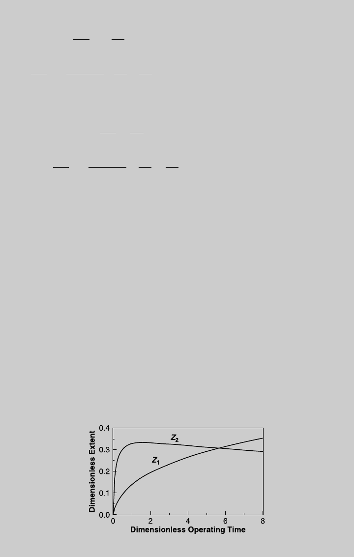
. Figure E9.1.1 shows the two reaction operating curves. Using
Eq. 9.1.15, we determine the species operating curves, N
j
(t
op
)/(N
tot
)
0
,
shown in the Figure E9.1.2.
c. We compare the species curves of the two products to those of an ideal batch
reactor (design equations derived below). Figure E9.1.3 shows the curves of
the desired product V, and Figure E9.1.4 shows the curves of the undesirable
product W. An examination of the two figures indicates that additional
amount of desirable product V can be obtained by semibatch operation
over a longer operating times. From the species operating curves,
N
A
(t
op
)=(N
tot
)
0
¼ 0:1 (90% conversion of A) is reached at t
op
¼ 4.4,
which corresponds to 44 min. At this t
op
, N
V
(t
op
)=(N
tot
)
0
¼ 0:309 and
N
W
(t
op
)=(N
tot
)
0
¼ 0:296 which correspond to 247.2 and 236.8 mol, respect-
ively. Similarly, for isothermal batch operation, N
A
(t)=(N
tot
)
0
¼ 0:1is
reached at t
op
¼ 0.56, which corresponds to 5.6 min. At this operating
Figure E9.1.1 Reaction operating curves—semibatch.
9.1 SEMIBATCH REACTORS 389