Neamen D. Microelectronics: Circuit Analysis and Design

Подождите немного. Документ загружается.

148 Part 1 Semiconductor Devices and Basic Applications

Solution: From the circuit shown in Figure 3.25(b) and Equation (3.12), we have

= V



+ R





20 + 30



(5) = 2V

Assuming the transistor is biased in the saturation region, the drain current is

= K

− V

)

= (0.1)(2 −1)

= 0.1mA

and the drain-to-source voltage is

= V

− I

= 5 −(0.1)(20) = 3V

The power dissipated in the transistor is

= I

= (0.1)(3) = 0.3mW

Comment: Because

= 3V> V

(sat) = V

− V

= 2 −1 = 1V

, the tran-

sistor is indeed biased in the saturation region and our analysis is valid.

The dc analysis produces the quiescent values (Q-points) of drain current and

drain-to-source voltage, usually indicated by

and

DSQ

EXERCISE PROBLEM

Ex 3.3: The transistor in Figure 3.25(a) has parameters

= 0.35

V and

= 25 μ

A/V

. The circuit parameters are

= 2.2

= 355 k,

= 245 k

, and

= 100 k

. Find

, V

, and

. (Ans.

= 7.52 μA,

= 0.898 V, V

= 1.45 V

)

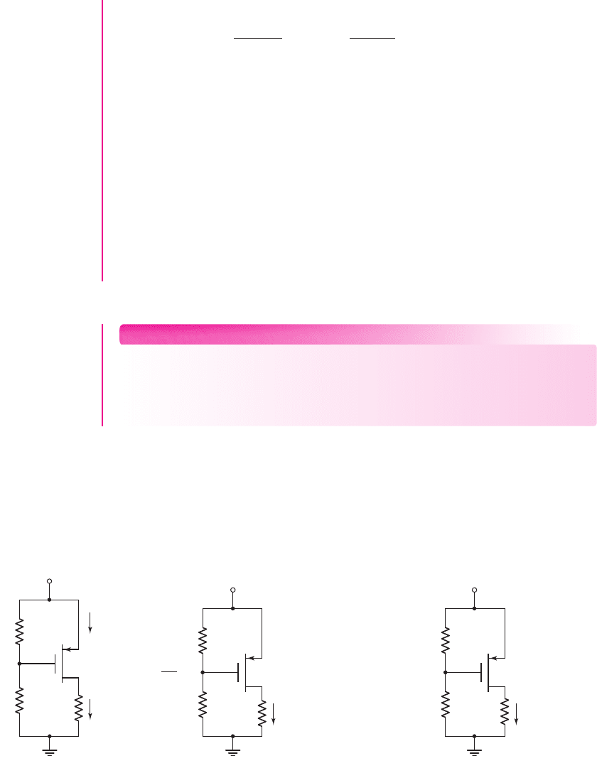
Figure 3.26 (a) shows a common-source circuit with a p-channel enhancement-

mode MOSFET. The source terminal is tied to

, which becomes signal ground

in the ac equivalent circuit. Thus the terminology common-source applies to this

circuit.

–

= 5 V

7.5 kΩ

= 50 kΩ

–

= 5 – (0.578)(7.5)

= 0.665 V < V

(sat)

2.5 V

= 0.578 mA

(Not correct)

= 5 V

7.5 kΩ

= 50 kΩ

–

= 5 – (0.515)(7.5)

= 1.14 V

2.5 V

= 0.515 mA

(Correct)

= 2.5 V

= (5)

()

100

= 2.5 V

(a) (b) (c)

Figure 3.26 (a) A PMOS common-source circuit, (b) the PMOS common-source circuit for

Example 3.4 showing current and voltage values when the saturation-region bias assumption

is incorrect, and (c) the circuit for Example 3.4 showing current and voltage values when the

nonsaturation-region bias assumption is correct

nea80644_ch03_125-204.qxd 06/08/2009 08:37 PM Page 148 F506 Hard disk:Desktop Folder:MHDQ134-03:

Chapter 3 The Field-Effect Transistor 149

The dc analysis is essentially the same as for the n-channel MOSFET circuit.

The gate voltage is



+ R



)

(3.16)

and the source-to-gate voltage is

= V

− V

(3.17)

Assuming that

< V

, or

> |V

, and that the device is biased in the

saturation region, the drain current is given by

= K

+ V

)

(3.18)

and the source-to-drain voltage is

= V

− I

(3.19)

> V

(sat) = V

+ V

, then the transistor is indeed biased in the

saturation region, as we have assumed. However, if

< V

(sat)

, the transistor is

biased in the nonsaturation region.

EXAMPLE 3.4

Objective: Calculate the drain current and source-to-drain voltage of a common-

source circuit with a p-channel enhancement-mode MOSFET.

Consider the circuit shown in Figure 3.26(a). Assume that

= R

= 50 k

= 5V

= 7.5k

=−0.8V

, and

= 0.2mA/V

Solution: From the circuit shown in Figure 3.26(b) and Equation (3.16), we have



+ R



) =



50 + 50



(5) = 2.5V

The source-to-gate voltage is therefore

= V

− V

= 5 −2.5 = 2.5V

Assuming the transistor is biased in the saturation region, the drain current is

= K

+ V

)

= (0.2)(2.5 −0.8)

= 0.578 mA

and the source-to-drain voltage is

= V

− I

= 5 −(0.578)(7.5) = 0.665 V

Since

= 0.665 V

is not greater than

(sat) = V

+ V

= 2.5 −0.8 =

1.7V

, the p-channel MOSFET is not biased in the saturation region, as we initially

assumed.

In the nonsaturation region, the drain current is given by

= K



2(V

+ V

− V



and the source-to-drain voltage is

= V

− I

Combining these two equations, we obtain

= K

[2(V

+ V

)(V

− I

) − (V

− I

)

]

nea80644_ch03_125-204.qxd 06/08/2009 08:37 PM Page 149 F506 Hard disk:Desktop Folder:MHDQ134-03:

150 Part 1 Semiconductor Devices and Basic Applications

= (0.2)[2(2.5 −0.8)(5 − I

(7.5)) − (5 − I

(7.5))

]

Solving this quadratic equation for

, we ﬁnd

= 0.515 mA

We also ﬁnd that

= 1.14 V

Therefore,

< V

(sat)

, which veriﬁes that the transistor is biased in the nonsat-

uration region.

Comment: In solving the quadratic equation for

, we ﬁnd a second solution that

yields

= 2.93 V.

However, this value of

is greater than

(sat)

, so it is not

a valid solution since we assumed the transistor to be biased in the nonsaturation

region.

EXERCISE PROBLEM

Ex 3.4: The transistor in Figure 3.26(a) has parameters

=−0.6V

and

0.2mA/V

. The circuit is biased at

= 3.3V.

Assume



= 300 k

. De-

sign the circuit such that

= 0.5mA

and

SDQ

= 2.0V

. (Ans.

= 885 k,

= 454 k, R

= 2.6k)

COMPUTER ANALYSIS EXERCISE

PS 3.1: Verify the results of Example 3.4 with a PSpice analysis.

As Example 3.4 illustrated, we may not know initially whether a transistor is

biased in the saturation or nonsaturation region. The approach involves making an

educated guess and then verifying that assumption. If the assumption proves incor-

rect, we must then change it and reanalyze the circuit.

In linear ampliﬁers containing MOSFETs, the transistors are biased in the satu-

ration region.

DESIGN EXAMPLE 3.5

Objective: Design a MOSFET circuit biased with both positive and negative volt-

ages to meet a set of speciﬁcations.

Speciﬁcations: The circuit conﬁguration to be designed is shown in Figure 3.27.

Design the circuit such that

= 0.5mA

and

DSQ

= 4V

Choices: Standard resistors are to be used in the final design. A transistor with

nominal parameters of



= 80 μA/V

(W/L) = 6.25

,and

= 1.2V

available.

Solution: Assuming the transistor is biased in the saturation region, we have

= K

− V

)

. The conduction parameter is





0.080



(6.25) = 0.25 mA/V

= +5 V

–

= –5 V

= 50 kΩ

Figure 3.27 Circuit conﬁgu-

ration for Example 3.5

nea80644_ch03_125-204.qxd 06/08/2009 08:37 PM Page 150 F506 Hard disk:Desktop Folder:MHDQ134-03:

Chapter 3 The Field-Effect Transistor 151

Solving for the gate-to-source voltage, we ﬁnd the required gate-to-source voltage to

induce the speciﬁed drain current.



+ V



0.5

0.25

+1.2

= 2.614 V

Since the gate current is zero, the gate is at ground potential. The voltage at the source

terminal is then

=−V

=−2.614 V

. The value of the source resistor is found from

− V

−

−2.614 − (−5)

0.5

= 4.77 k

The voltage at the drain terminal is determined to be

= V

+ V

=−2.614 + 4 = 1.386 V

The value of the drain resistor is

− V

5 − 1.386

0.5

= 7.23 k

We may note that

= 4 V > V

(sat) = V

− V

= 2.61 −1.2 = 1.41 V

which means that the transistor is indeed biased in the saturation region.

Trade-offs: The closest standard resistor values are

= 4.7k

and

= 7.5k

We may ﬁnd the gate-to-source voltage from

+ I

−5 = 0

where

= K

− V

)

Using the standard resistor values, we ﬁnd

= 2.622 V, I

= 0.506 mA,

and

DSQ

= 3.83 V.

In this case, the drain current is within 1.2 percent of the design speci-

ﬁcation and the drain-to-source voltage is within 4.25 percent of the design speciﬁcation.

Comment: It is important to keep in mind that the current into the gate terminal is

zero. In this case, then, there is zero voltage drop across the

resistor.

Design Pointer: In an actual circuit design using discrete elements, we need to

choose standard resistor values that are closest to the design values. In addition, the

discrete resistors have tolerances that need to be taken into account. In the ﬁnal de-

sign, then, the actual drain current and drain-to-source voltage are somewhat differ-

ent from the speciﬁed values. In many applications, this slight deviation from the

speciﬁed values will not cause a problem.

nea80644_ch03_125-204.qxd 06/08/2009 08:37 PM Page 151 F506 Hard disk:Desktop Folder:MHDQ134-03:

–

= –2.5 V

= 2.5 V

–

Figure 3.29 Circuit conﬁgu-

ration for Example 3.6

152 Part 1 Semiconductor Devices and Basic Applications

Figure 3.28

Circuit for

Exercise Ex 3.5

4 kΩ

60 kΩ

30 kΩ

–

= –2.5 V

= +2.5 V

EXERCISE PROBLEM

Ex 3.5: For the transistor in the circuit in Figure 3.28, the nominal parameter val-

ues are

= 0.6V

and

= 0.5mA/V

. (a) Determine the quiescent values

GSQ

, and

DSQ

. (b) Determine the range in

and

values for a

±5

percent variation in

and

. (Ans. (a)

GSQ

= 1.667 V, I

= 0.5689 mA,

DSQ

= 2.724 V;

(b)

0.5105 ≤ I

≤ 0.6314 mA, 2.474 ≤ V

≤ 2.958 V)

Now consider an example of a p-channel device biased with both positive and nega-

tive voltages.

DESIGN EXAMPLE 3.6

Objective: Design a circuit with a p-channel MOSFET that is biased with both neg-

ative and positive supply voltages and that contains a source resistor

to meet a set

of speciﬁcations.

Speciﬁcations: The circuit to be designed is shown in Figure 3.29. Design the circuit

such that

= 100 μA, V

SDQ

= 3V,

and

= 0.8V.

Note that

is the volt-

age across the source resistor

. The value of the larger bias resistor, either

, is to be

200 k

Choices: A transistor with nominal parameter values of

= 100 μA/V

and

=−0.4V

is available. The conduction parameter may vary by

±5

percent.

Solution: Assuming that the transistor is biased in the saturation region, we have

= K

+ V

)

. Solving for the source-to-gate voltage, we ﬁnd the required

value of source-to-gate voltage to be



− V



100

−(−0.4)

= 1.4V

We may note that the design value of

SDQ

= 3V> V

SDQ

(

sat

)

= V

SGQ

+ V

= 1.4 −0.4 = 1V

so that the transistor will be biased in the saturation region.

The voltage at the gate with respect to ground potential is found to be

= V

− V

= 2.5 −0.8 −1.4 = 0.3V

With

> 0

, the resistor

will be the larger of the two bias resistors, so set

= 200 k

. The current through

is then

Bias

− V

−

0.3 − (−2.5)

200

= 0.014 mA

Since the current through

is the same, we can ﬁnd the value of

to be

− V

Bias

2.5 − 0.3

0.014

which yields

= 157 k

nea80644_ch03_125-204.qxd 06/08/2009 08:37 PM Page 152 F506 Hard disk:Desktop Folder:MHDQ134-03:

Chapter 3 The Field-Effect Transistor 153

The source resistor value is found from

0.8

0.1

= 8k

The voltage at the drain terminal is

= V

− V

= 2.5 −0.8 −3 =−1.3V

Then the drain resistor value is found as

− V

−

−1.3 − (−2.5)

0.1

= 12 k

Trade-offs: If the conduction parameter

varies by

±5

%, the quiescent drain cur-

rent

and the source-to-drain voltage

SDQ

will change. Using the resistor values

found in the previous design, we ﬁnd the following:

SGQ

SDQ

95 μA/V

1.416 V 98.0 μA3.04 V

105 μA/V

1.385 V 101.9 μA2.962 V

±5% ±1.14% ±2% ±1.33%

Comment: We may note that the variation in the Q-point values is smaller that the

variation in

. Including the source resistor

tends to stabilize the

-point.

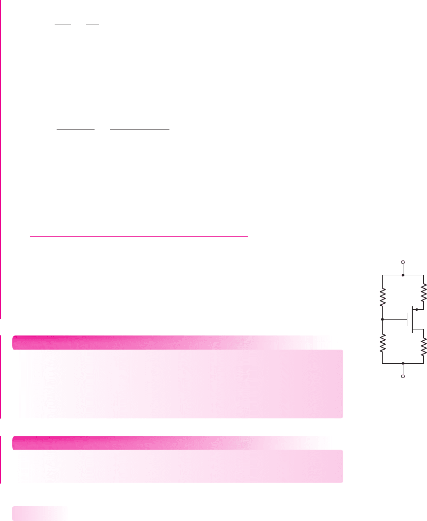
EXERCISE PROBLEM

Ex 3.6: Consider the circuit shown in Figure 3.30. The nominal transistor

parameters are

=−0.30 V

and

= 120 μA/V

. (a) Calculate

and

. (b) Determine the variation in

if the threshold voltage varies by

±5

percent. (Ans. (a)

= 1.631 V, I

= 0.2126 mA, V

= 3.295 V;

(b)

0.2091 ≤ I

≤ 0.2160 mA)

COMPUTER ANALYSIS EXERCISE

PS 3.2 Verify the circuit design in Example 3.6 with a PSpice simulation. Also

investigate the change in Q-point values with

±10

percent variations in resistor values.

Load Line and Modes of Operation

The load line is helpful in visualizing the region in which the MOSFET is biased.

Consider again the common-source circuit shown in Figure 3.25(b). Writing a

Kirchhoff’s voltage law equation around the drain-source loop results in Equa-

tion (3.14), which is the load line equation, showing a linear relationship between

the drain current and drain-to-source voltage.

3.2.2

Figure 3.30 Figure for

Exercise Ex 3.6

+2.2 V

–2.2 V

6 kΩ

42 kΩ

255 kΩ

345 kΩ

nea80644_ch03_125-204.qxd 06/08/2009 08:37 PM Page 153 F506 Hard disk:Desktop Folder:MHDQ134-03:

154 Part 1 Semiconductor Devices and Basic Applications

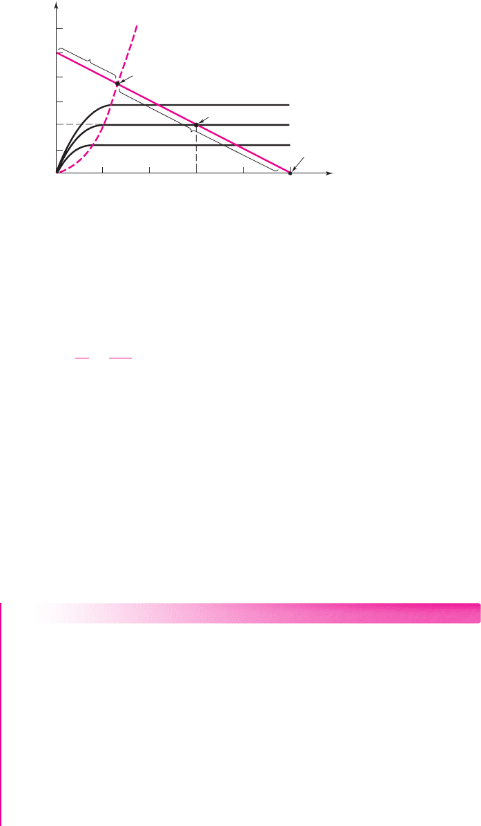
Figure 3.31 shows the

(sat) characteristic for the transistor described in

Example 3.3. The load line is given by

= V

− I

= 5 − I

(20)

(3.20(a))

−

(mA)

(3.20(b))

and is also plotted in the ﬁgure. The two end points of the load line are determined in

the usual manner. If

= 0

, then

= 5V

; if

= 0

, then

= 5/20 =

0.25 mA.

The Q-point of the transistor is given by the dc drain current and drain-to-

source voltage, and it is always on the load line, as shown in the ﬁgure. A few

transistor characteristics are also shown on the ﬁgure.

If the gate-to-source voltage is less than V

, the drain current is zero and the

transistor is in cutoff. As the gate-to-source voltage becomes just greater than V

the transistor turns on and is biased in the saturation region. As V

increases, the

Q-point moves up the load line. The transition point is the boundary between

the saturation and nonsaturation regions and is deﬁned as the point where

(sat) = V

− V

As V

increases above the transition point value, the tran-

sistor becomes biased in the nonsaturation region.

EXAMPLE 3.7

Objective: Determine the transition point parameters for a common-source circuit.

Consider the circuit shown in Figure 3.25(b). Assume transistor parameters of

= 1V

and

= 0.1mA/V

Solution: At the transition point,

= V

(sat) = V

− V

= V

− I

The drain current is still

= K

− V

)

Combining the last two equations, we obtain

− V

= V

− K

− V

)

(mA)

(sat) = v

– V

GSQ

= 2 V

Saturation region

Nonsaturation

region

Transition point

Q-point

Cutoff

0.05

0 12345

0.10

0.15

0.20

0.25

0.30

Figure 3.31 Transistor characteristics,

(sat) curve, load line, and Q-point for the NMOS

common-source circuit in Figure 3.25(b)

nea80644_ch03_125-204.qxd 06/08/2009 08:37 PM Page 154 F506 Hard disk:Desktop Folder:MHDQ134-03:

Chapter 3 The Field-Effect Transistor 155

Rearranging this equation produces

− V

)

+(V

− V

) − V

= 0

(0.1)(20)(V

− V

)

+(V

− V

) − 5 = 0

Solving the quadratic equation, we ﬁnd that

− V

= 1.35 V = V

Therefore,

= 2.35 V

and

= (0.1)(2.35 −1)

= 0.182 mA

Comment: For

< 2.35 V

, the transistor is biased in the saturation region; for

> 2.35 V

, the transistor is biased in the nonsaturation region.

EXERCISE PROBLEM

Ex 3.7: Consider the circuit in Figure 3.30. Using the nominal transistor parame-

ters described in Exercise Ex 3.6, draw the load line and determine the transition

point parameters. (Ans.

= 2.272 V, I

= 0.4668 mA, V

= 1.972 V)

Problem-Solving Technique: MOSFET DC Analysis

Analyzing the dc response of a MOSFET circuit requires knowing the bias con-

dition (saturation or nonsaturation) of the transistor. In some cases, the bias

condition may not be obvious, which means that we have to guess the bias condi-

tion, then analyze the circuit to determine if we have a solution consistent with our

initial guess. To do this, we can:

1. Assume that the transistor is biased in the saturation region, in which case

> V

> 0

, and

≥ V

(sat)

2. Analyze the circuit using the saturation current-voltage relations.

3. Evaluate the resulting bias condition of the transistor. If the assumed parame-

ter values in step 1 are valid, then the initial assumption is correct. If

< V

, then the transistor is probably cutoff, and if

< V

(sat)

, the

transistor is likely biased in the nonsaturation region.

4. If the initial assumption is proved incorrect, then a new assumption must be

made and the circuit reanalyzed. Step 3 must then be repeated.

Additional MOSFET Conﬁgurations: DC Analysis

There are other MOSFET circuits, in addition to the basic common-source circuits

just considered, that are biased with the basic four-resistor conﬁguration.

However, MOSFET integrated circuit ampliﬁers are generally biased with constant

current sources. Example 3.8 demonstrates this technique using an ideal current source.

3.2.3

nea80644_ch03_125-204.qxd 06/08/2009 08:37 PM Page 155 F506 Hard disk:Desktop Folder:MHDQ134-03:

156 Part 1 Semiconductor Devices and Basic Applications

DESIGN EXAMPLE 3.8

Objective: Design a MOSFET circuit biased with a constant-current source to meet

a set of speciﬁcations.

Speciﬁcations: The circuit conﬁguration to be designed is shown in Figure 3.32(a).

Design the circuit such that the quiescent values are

= 250 μA

and

= 2.5V

Choices: A transistor with nominal values of

= 0.8V



= 80 μA/V

, and

W/L = 3

is available. Assume



varies by

±5

percent.

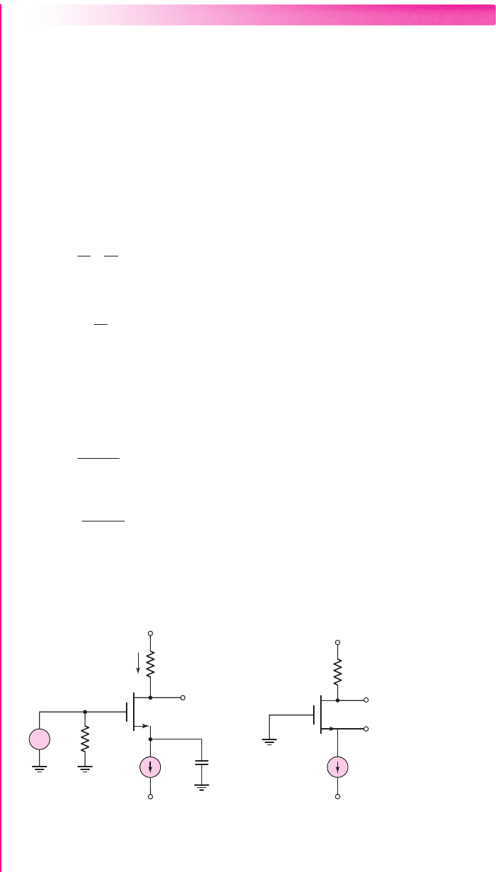
Solution: The dc equivalent circuit is shown in Figure 3.32(b). Since

= 0

, the

gate is at ground potential and there is no current through

. We have that

= I

= 250 μA.

Assuming the transistor is biased in the saturation region, we have



− V

)

250 =





· (3)(V

−0.8)

which yields

= 2.24 V

The voltage at the source terminal is

=−V

=−2.24 V

The drain current can also be written as

5 − V

For

= 2.5V

, we have

5 − 2.5

0.25

= 10 k

The drain-to-source voltage is

= V

− V

= 2.5 −(−2.24) = 4.74 V

+5 V

–5 V –5 V

–

(a) (b)

–

Figure 3.32 (a) NMOS common-source circuit biased with a constant-current source and (b)

equivalent dc circuit

nea80644_ch03_125-204.qxd 06/08/2009 09:10 PM Page 156 F506 Tempwork:Dont' Del Rakesh:June:Rakesh 06-08-09:MHDQ134-03 Folder:

Chapter 3 The Field-Effect Transistor 157

Since

= 4.74 V > V

(sat) = V

− V

= 2.24 −0.8 = 1.44 V

, the transis-

tor is biased in the saturation region, as initially assumed.

Trade-offs: Note that even if



changes, the drain current remains constant. For

76 ≤ k



≤ 84 μA/V

, the variation in

GSQ

2.209 ≤ V

GSQ

≤ 2.281 V

and the

variation in

DSQ

4.709 ≤ V

DSQ

≤ 4.781 V

. The variation in

DSQ

±0.87

per-

cent even with a

±5

percent variation in



. This stability effect is one advantage of

using constant current biasing.

Comment: MOSFET circuits can be biased by using constant-current sources,

which in turn are designed by using other MOS transistors, as we will see. Biasing

with current sources tends to stabilize circuits against variations in device or circuit

parameters.

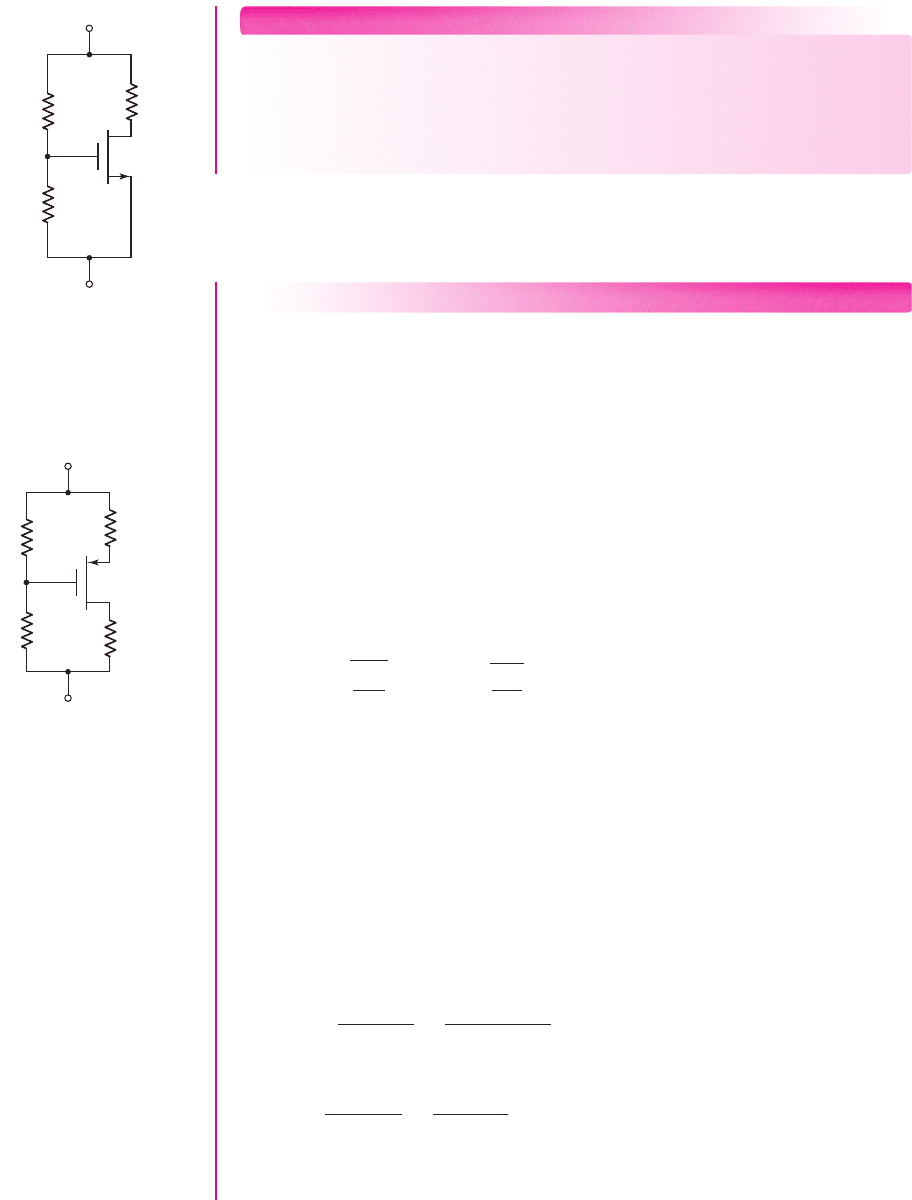
EXERCISE PROBLEM

Ex 3.8: (a) Consider the circuit shown in Figure 3.33. The transistor parameters

are

=−0.40

V and

= 30 μ

A/V

. Design the circuit such that

= 60 μ

A and

SDQ

= 2.5

V. (b) Determine the variation in

-point values if

the

and

parameters vary by

±5

percent. (Ans. (a)

= 19.77



= 38.57



; (b)

58.2 ≤ I

≤ 61.08 μ

2.437 ≤ V

SDQ

≤ 2.605

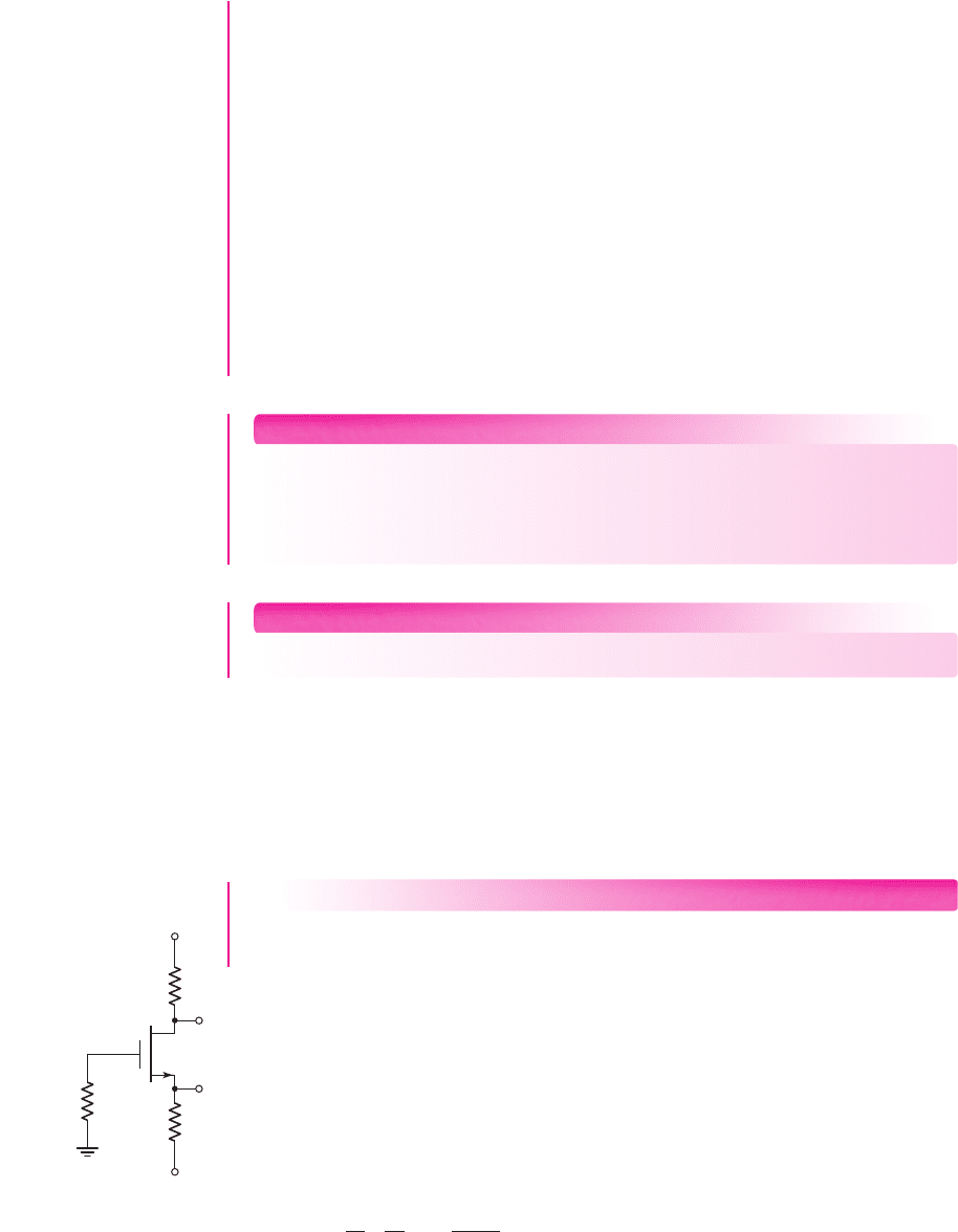
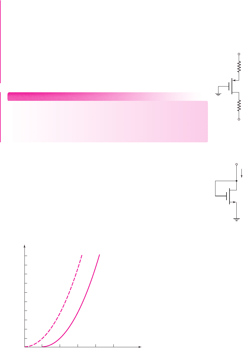
n-Channel Enhancement-Load Device

An enhancement-mode MOSFET connected in a conﬁguration such as that shown in

Figure 3.34 can be used as a nonlinear resistor. A transistor with this connection is

called an enhancement-load device. Since the transistor is an enhancement mode

device,

> 0

. Also, for this circuit,

= v

(sat) = v

− V

, which

means that the transistor is always biased in the saturation region. The general i

ver-

sus

characteristics can then be written as

= K

− V

)

= K

− V

)

(3.21)

Figure 3.35 shows a plot of Equation (3.21) for the case when

= 1mA/V

and

= 1V

+3 V

–3 V

Figure 3.33 Circuit for

Exercise Ex 3.8

Transistor

characteristics

(V)

(mA)

(sat) = v

– V

0 12345

Figure 3.35 Current–voltage characteristic of an enhancement load device

–

Figure 3.34 Enhancement-

mode NMOS device with the

gate connected to the drain

nea80644_ch03_125-204.qxd 06/08/2009 08:37 PM Page 157 F506 Hard disk:Desktop Folder:MHDQ134-03: