Schmuller J. Statistical Analysis with Excel For Dummies
Подождите немного. Документ загружается.

99
Chapter 5: Deviating from the Average
Sample variance
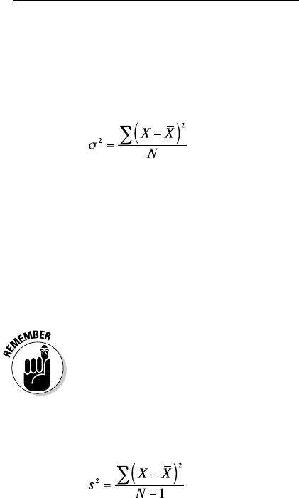
Earlier, I mentioned that you use this formula to calculate population
variance:
I also said that sample variance is a little different. Here’s the difference.
If your set of numbers is a sample drawn from a large population, you’re
probably interested in using the variance of the sample to estimate the vari-
ance of the population.
The formula you used for the variance doesn’t quite work as an estimate of
the population variance. Although the sample mean works just fine as an
estimate of the population mean, this doesn’t hold true with variance, for rea-
sons way beyond the scope of this book.
How do you calculate a good estimate of the population variance? It’s pretty
easy. You just use N-1 in the denominator rather than N. (Again, for reasons
way beyond our scope.)
Also, because we’re working with a characteristic of a sample (rather than
of a population), we use the English equivalent of the Greek letter — s rather
than σ. This means that the formula for the sample variance is
The value of s
2
, given the squared deviations in our set of five numbers is
(4 + 1 + 16 + 4 + 9)/4 = 34/4 = 8.5
So, if these numbers
50, 47, 52, 46, 45
are an entire population, their variance is 6.4. If they’re a sample drawn from
a larger population, our best estimate of that population’s variance is 8.5.
10 454060-ch05.indd 9910 454060-ch05.indd 99 4/21/09 7:21:14 PM4/21/09 7:21:14 PM
100
Part II: Describing Data
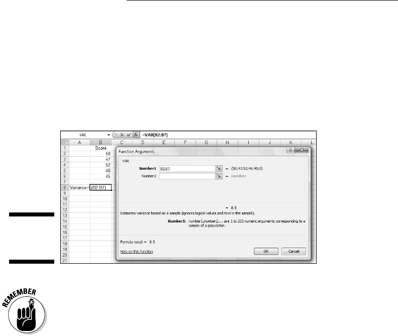
VAR and VARA
The worksheet functions VAR and VARA calculate the sample variance.
Figure 5-3 shows the Function Arguments dialog box for VAR with 50, 47, 52,
46, 45 entered into cells B2 through B6. Cell B7 is part of the cell range, but I
left it empty.
Figure 5-3:
Working
with VAR.
The relationship between VAR and VARA is the same as the relationship
between VARP and VARPA: VAR ignores cells that contain logical values
(TRUE and FALSE) and text. VARA includes those cells. Once again, TRUE
evaluates to 1.0 and FALSE evaluates to 0. Text in a cell causes VARA to see
that cell’s value as 0.
This is why I left B7 blank. If you experiment a bit with VARA and logical
values or text in B7, you’ll see exactly what VARA does.
Back to the Roots: Standard Deviation
After you calculate the variance of a set of numbers, you have a value whose
units are different from your original measurements. For example, if your
original measurements are in inches, their variance is in square inches. This
is because you square the deviations before you average them.
Often, it’s more intuitive if you have a variation statistic that’s in the same
units as the original measurements. It’s easy to turn variance into that kind
of statistic. All you have to do is take the square root of the variance.
10 454060-ch05.indd 10010 454060-ch05.indd 100 4/21/09 7:21:14 PM4/21/09 7:21:14 PM
101
Chapter 5: Deviating from the Average
Like the variance, this square root is so important that we give it a special
name: standard deviation.
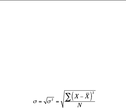
Population standard deviation
The standard deviation of a population is the square root of the population
variance. The symbol for the population standard deviation is σ (sigma). Its
formula is
For these measurements (in inches)
50, 47, 52, 46, 45
the population variance is 6.8 square inches, and the population standard
deviation is 2.61 inches (rounded off).
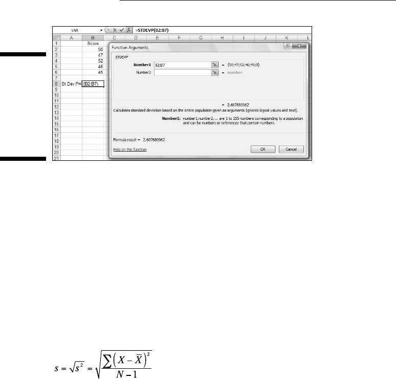
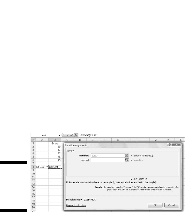
STDEVP and STDEVPA
The Excel worksheet functions STDEVP and STDEVPA calculate the popula-
tion standard deviation. After entering your numbers into your worksheet
and selecting a cell
1. Type your data into an array and select a cell for the result.
2. In the Statistical Functions menu, select STDEVP to open the STDEVP
Function Arguments dialog box.
3. In the Function Arguments dialog box, type the appropriate values for
the arguments.
After you enter the data array, the dialog box shows the value of the pop-
ulation standard deviation for the numbers in the data array. Figure 5-4
shows this.
10 454060-ch05.indd 10110 454060-ch05.indd 101 4/21/09 7:21:14 PM4/21/09 7:21:14 PM
102
Part II: Describing Data
Figure 5-4:
The
Function
Arguments
dialog box
for STDEVP,
along with
the data.
4. Click OK to close the dialog box and put the result into the
selected cell.
Like VARPA, STDEVPA uses any logical values and text values it finds when
it calculates the population standard deviation. TRUE evaluates to 1.0 and
FALSE evaluates to 0. Text in a cell gives that cell a value of 0.
Sample standard deviation
The standard deviation of a sample — an estimate of the standard deviation
of a population — is the square root of the sample variance. Its symbol is s
and its formula is
For these measurements (in inches)
50, 47, 52, 46, 45
the population variance is 8.4 square inches, and the population standard
deviation is 2.92 inches (rounded off).
STDEV and STDEVA
The Excel worksheet functions STDEV and STDEVA calculate the sample stan-
dard deviation. To work with STDEV
10 454060-ch05.indd 10210 454060-ch05.indd 102 4/21/09 7:21:14 PM4/21/09 7:21:14 PM
103
Chapter 5: Deviating from the Average
1. Type your data into an array and select a cell for the result.
2. In the Statistical Functions menu, select STDEV to open the STDEV
Function Arguments dialog box.
3. In the Function Arguments dialog box, type the appropriate values for
the arguments.
With the data array entered, the dialog box shows the value of the popu-
lation standard deviation for the numbers in the data array. Figure 5-5
shows this.
4. Click OK to close the dialog box and put the result into the
selected cell.
STDEVA uses text and logical values in its calculations. Cells with text have
values of 0, and cells whose values are FALSE also evaluate to 0. Cells that
evaluate to TRUE have values of 1.0.
Figure 5-5:
The
Function
Arguments
dialog box
for STDEV.
The missing functions: STDEVIF and
STDEVIFS
Here’s a rule of thumb: Whenever you present a mean, provide a standard
deviation. Use AVERAGE and STDEV in tandem.
Remember that Excel 2007 offers two new functions, AVERAGEIF and
AVERAGEIFS, for calculating means conditionally. (See Chapter 4.) Two
additional new functions would have been helpful: STDEVIF and STDEVIFS
for calculating standard deviations conditionally when you calculate means
conditionally.
10 454060-ch05.indd 10310 454060-ch05.indd 103 4/21/09 7:21:14 PM4/21/09 7:21:14 PM

104
Part II: Describing Data
Excel 2007, however, doesn’t provide these functions. Instead, I show you
a couple of workarounds that enable you to calculate standard deviations
conditionally.
The workarounds filter out data that meet a set of conditions, and then
calculate the standard deviation of the filtered data. Figure 5-6 shows what
I mean. The data are from the fictional psychology experiment I describe in
Chapter 4.
Here, once again, is the description:
A person sits in front of a screen and a color-filled shape appears. The color
is either red or green and the shape is either a square or a circle. The combi-
nation for each trial is random, and all combinations appear an equal number
of times. In the lingo of the field, each appearance of a color-filled shape is
called a trial. So the worksheet shows the outcomes of 16 trials.
Figure 5-6:
Filtering
data to
calculate
standard
deviation
conditionally.
The person sitting in front of the screen presses a button as soon as he or she
sees the shape. Column A presents the trial number. Columns B and C show
the color and shape, respectively, presented on that trial. Column D (labeled
RT_msec) presents one person’s reaction time in milliseconds (thousandths
of a second) for each trial. So, for example, row 2 tells you that on the first trial,
a red circle appeared and the person responded in 410 msec (milliseconds).
For each column, I defined the name in the top cell of the column to refer
to the data in that column. If you don’t remember how to do that, reread
Chapter 2.
Cell D19 displays the overall average of RT_msec. The formula for that aver-
age, of course, is
=AVERAGE(RT_msec)
10 454060-ch05.indd 10410 454060-ch05.indd 104 4/21/09 7:21:15 PM4/21/09 7:21:15 PM

105
Chapter 5: Deviating from the Average
Cell D20 shows the average for all trials on which a circle appeared. The for-
mula that calculates that conditional average is
=AVERAGEIF(Shape,”Circle”,RT_msec)
Cell D21 presents the average for trials on which a green square appeared.
That formula is
=AVERAGEIFS(RT_msec, Color,”Green”, Shape,”Square”)
Columns H and K hold filtered data. Column H shows the data for trials that
displayed a circle. Cell H19 presents the standard deviation for those trials
and is the equivalent of
=STDEVIF(Shape,”Circle”,RT_msec)
if this function existed.
Column K shows the data for trials that displayed a green square. Cell K19
presents the standard deviation for those trials, and is the equivalent of
=STDEVIFS(RT_msec, Color,”Green”,Shape,”Square”)
if that function existed.
How did I filter the data? I’ll let you in on it in a moment, but first I have to tell
you about . . .
A little logic
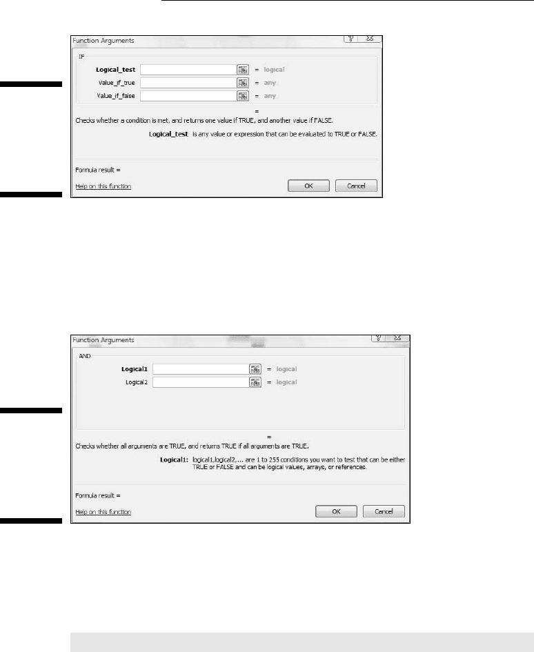
In order to proceed, you have to know about two of Excel’s logic functions: IF
and AND. You access them by clicking
Formulas | Logical Functions
and selecting them from the Logical Functions menu.
IF takes three arguments:
✓ A logical condition to be satisfied
✓ The action to take if the logical condition is satisfied (that is, if the value
of the logical condition is TRUE)
✓ An optional argument that specifies the action to take if the logical
condition is not satisfied (that is, if the value of the logical condition
is FALSE)
Figure 5-7 shows the Function Arguments dialog box for IF.
10 454060-ch05.indd 10510 454060-ch05.indd 105 4/21/09 7:21:15 PM4/21/09 7:21:15 PM
106
Part II: Describing Data
Figure 5-7:
The
Function
Arguments
dialog box
for IF.
AND can take up to 255 arguments. AND checks to see if all of its arguments
meet each specified condition — that is, if each condition is TRUE. If they all
do, AND returns the value TRUE. If not, AND returns FALSE.
Figure 5-8 shows the Function Arguments dialog box for AND.
Figure 5-8:
The
Function
Arguments
dialog box
for AND.
And now, back to the show
In this example, I use IF to set the value of a cell in column H to the corre-
sponding value in column D if the value in the corresponding cell in column C
is “Circle”. The formula in cell H2 is
=IF(C2=”Circle”,D2,” “)
If this were a phrase it would be, “If the value in C2 is ‘Circle’, then set the
value of this cell to the value in D2. If not, leave this cell blank.” Autofilling the
next 15 cells of column H yields the filtered data in column H in Figure 5-6.
The standard deviation in cell H19 is the value STDEVIF would have provided.
10 454060-ch05.indd 10610 454060-ch05.indd 106 4/21/09 7:21:15 PM4/21/09 7:21:15 PM

107
Chapter 5: Deviating from the Average
I could have omitted the third argument (the two double-quotes) without
affecting the value of the standard deviation. Without the third argument,
Excel fills in FALSE for cells that don’t meet the condition instead of leaving
them blank.
I use AND along with IF for the cells in column K. Each one holds the value
from the corresponding cell in column D if two conditions are true:
✓ The value in the corresponding cell in column B is “Green”
✓ The value in the corresponding cell in column C is “Square”
The formula for cell K2 is
=IF(AND(B2=”Green”,C2=”Square”),D2,” “)
If this was a phrase it would be, “If the value in B2 is ‘Green’ and the value in
C2 is ‘Square’, then set the value of this cell to the value in D2. If not, leave
this cell blank.” Autofilling the next 15 cells in column K results in the filtered
data in column K in Figure 5-6. The standard deviation in cell K19 is the value
STDEVIFS would have provided.
Related Functions
Before we move on, take a quick look at a couple of other variation-related
worksheet functions.
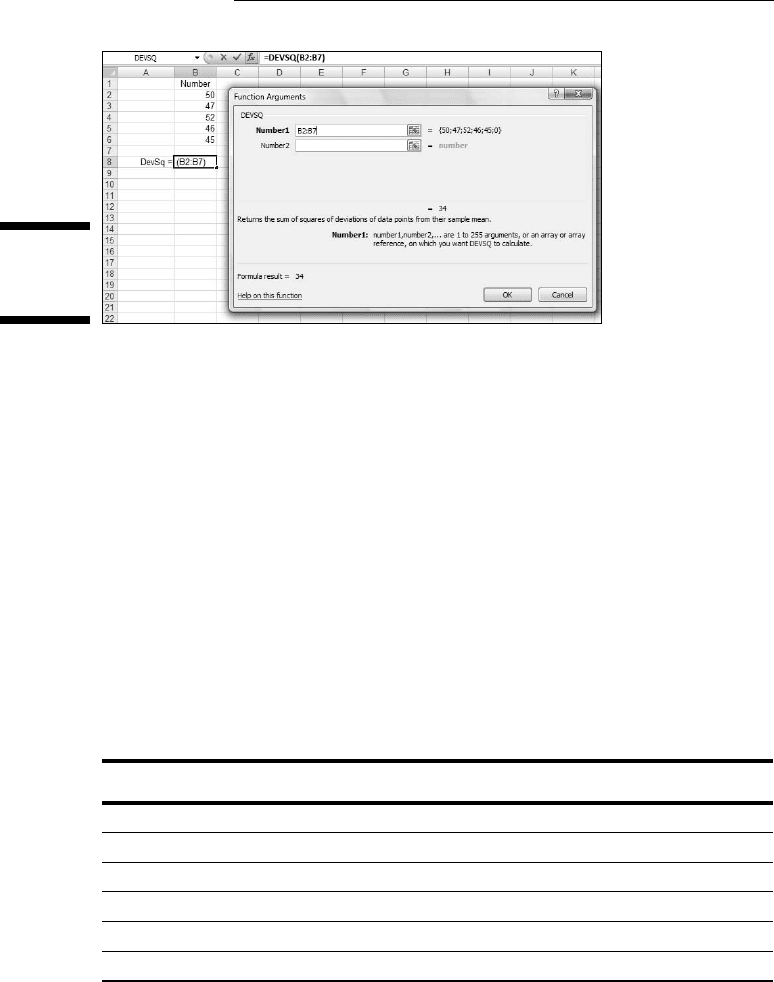
DEVSQ
DEVSQ calculates the sum of the squared deviations from the mean (without
dividing by N or by N-1). For these numbers
50, 47, 52, 46, 45
that’s 34, as Figure 5-9 shows.
10 454060-ch05.indd 10710 454060-ch05.indd 107 4/21/09 7:21:15 PM4/21/09 7:21:15 PM
108
Part II: Describing Data
Figure 5-9:
The DEVSQ
dialog box.
Average deviation
One more Excel function deals with deviations in a way other than squaring
them.
The variance and standard deviation deal with negative deviations by squar-
ing all the deviations before averaging them. How about if we just ignore the
minus signs? This is called taking the absolute value of each deviation. (That’s
the way mathematicians say “How about if we just ignore the minus signs?”).
If we do that for the heights
50, 47, 52, 46, 45
we can put the absolute values of the deviations into a table like Table 5-4.
Table 5-4 A Group of Numbers and Their Absolute Deviations
Height Height-Mean |Deviation|
50 50-48 2
47 47-48 1
52 52-48 4
46 46-48 2
45 45-48 3
10 454060-ch05.indd 10810 454060-ch05.indd 108 4/21/09 7:21:15 PM4/21/09 7:21:15 PM