Schmuller J. Statistical Analysis with Excel For Dummies

Подождите немного. Документ загружается.

179

Chapter 10: One-Sample Hypothesis Testing

t for One

In the preceding example, I worked with IQ scores. The population of IQ

scores is a normal distribution with a well-known mean and standard devia-

tion. This enabled me to work with the Central Limit Theorem and describe

the sampling distribution of the mean as a normal distribution. I was then

able to use z as the test statistic.

In the real world, however, you typically don’t have the luxury of working

with such well-defined populations. You usually have small samples, and

you’re typically measuring something that isn’t as well known as IQ. The

bottom line is that you often don’t know the population parameters, nor do

you know whether or not the population is normally distributed.

When that’s the case, you use the sample data to estimate the population

standard deviation, and you treat the sampling distribution of the mean as a

member of a family of distributions called the t-distribution. You use t as a test

statistic. In Chapter 9, I introduce this distribution, and mention that you dis-

tinguish members of this family by a parameter called degrees of freedom (df).

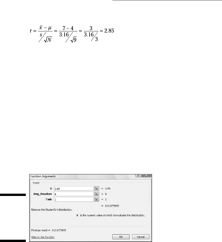
The formula for the test statistic is

Think of df as the denominator of the estimate of the population variance.

For the hypothesis tests in this section, that’s N-1, where N is the number of

scores in the sample. The higher the df, the more closely the t-distribution

resembles the normal distribution.

Here’s an example. FarKlempt Robotics, Inc., markets microrobots. They

claim their product averages four defects per unit. A consumer group

believes this average is higher. The consumer group takes a sample of 9

FarKlempt microrobots and finds an average of 7 defects, with a standard

deviation of 3.16. The hypothesis test is:

: μ ≤ 4

: μ > 4

α = .05

16 454060-ch10.indd 17916 454060-ch10.indd 179 4/21/09 7:29:23 PM4/21/09 7:29:23 PM

180

Part III: Drawing Conclusions from Data

The formula is:

Can you reject H

? The Excel function in the next section tells you.

TDIST

You use the worksheet function TDIST to decide whether or not your calcu-

lated t value is in the region of rejection. You supply a value for t, a value for

df, and determine whether the test is one-tailed or two-tailed. TDIST returns

the probability of obtaining a t value at least as high as yours if H

is true. If

that probability is less than your α, you reject H

The steps are:

1. Select a cell to store the result.

2. From the Statistical Functions menu, select TDIST to open the Function

Arguments dialog box for TDIST. (See Figure 10-4.)

Figure 10-4:

The

Function

Arguments

dialog box

for TDIST.

3. In the Function Arguments dialog box, enter the appropriate values

for the arguments.

The calculated t value goes in the X box. For this example, the calculated

t value is 2.85.

The degrees of freedom go in the Deg_freedom box. The degrees of free-

dom for this example is 8 (9 scores – 1).

16 454060-ch10.indd 18016 454060-ch10.indd 180 4/21/09 7:29:23 PM4/21/09 7:29:23 PM

181

Chapter 10: One-Sample Hypothesis Testing

In the Tails box, the idea is to type 1 (for a one-tailed test) or 2 (for a

two-tailed test). In this example, it’s a one-tailed test. After I typed 1, the

dialog box shows the probability in the tail of the t-distribution beyond

the t value.

4. Click OK to close the dialog box and put the answer in the selected cell.

The value in the dialog box in Figure 10-4 is less than .05, so the decision is to

reject H

Testing a Variance

So far, I’ve told you about one-sample hypothesis testing for means. You can

also test hypotheses about variances.

This sometimes comes up in the context of manufacturing. For example, sup-

pose FarKlempt Robotics, Inc, produces a part that has to be a certain length

with a very small variability. You can take a sample of parts, measure them,

find the sample variability and perform a hypothesis test against the desired

variability.

The family of distributions for the test is called chi-square. Its symbol is χ

. I

won’t go into all the mathematics. I’ll just tell you that, once again, df is the

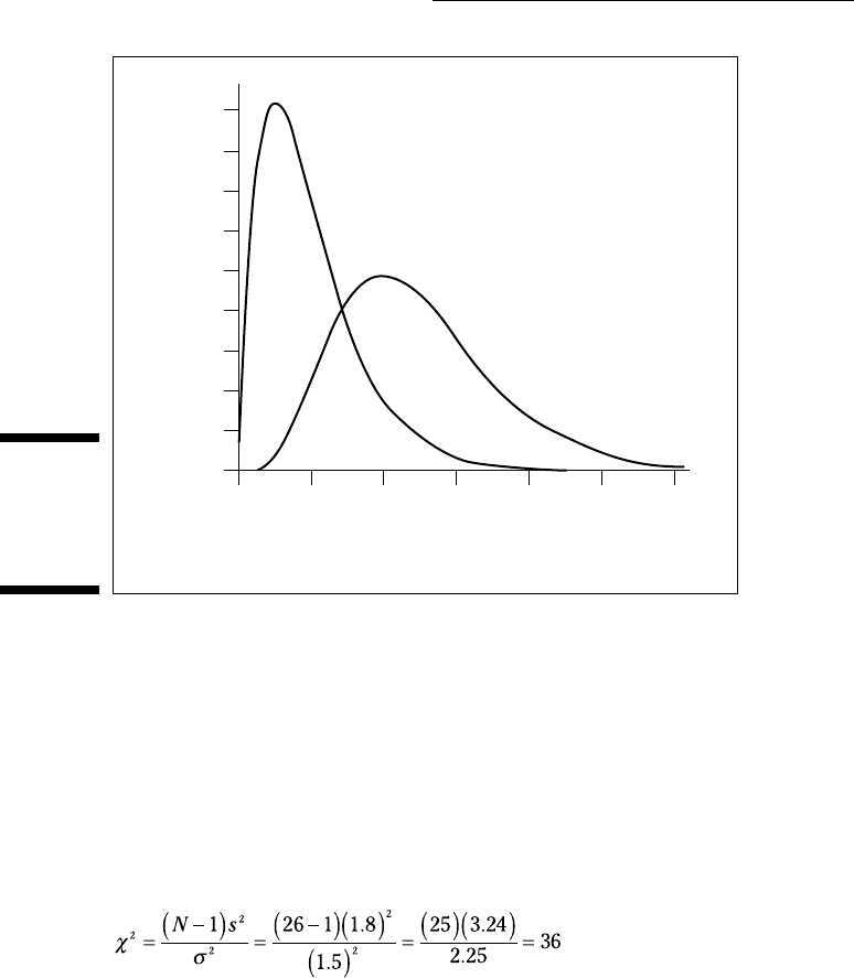
parameter that distinguishes one member of the family from another. Figure

10-5 shows two members of the chi-square family.

The formula for this test statistic is

N is the number of scores in the sample, s

is the sample variance, and σ

the population variance specified in H

With this test, you have to assume that what you’re measuring has a normal

distribution.

Suppose the process for the FarKlempt part has to have at most a standard

deviation of 1.5 inches for its length. (Notice I said standard deviation. This

allows me to speak in terms of inches. If I said variance the units would be

square inches.). After measuring a sample of 26 parts, you find a standard

deviation of 1.8 inches.

16 454060-ch10.indd 18116 454060-ch10.indd 181 4/21/09 7:29:24 PM4/21/09 7:29:24 PM

182

Part III: Drawing Conclusions from Data

Figure 10-5:

Two mem-

bers of the

chi-square

family.

f(x

)

16 df=4

df=10

04812162024

The hypotheses are:

: σ

≤ 2.25 (remember to square the “at-most” standard deviation of 1.5

inches)

: σ

> 2.25

α = .05

Working with the formula,

Can you reject H

? Read on.

CHIDIST

After calculating a value for your chi-square test statistic, you use the

CHIDIST worksheet function to make a judgment about it. You supply the

16 454060-ch10.indd 18216 454060-ch10.indd 182 4/21/09 7:29:24 PM4/21/09 7:29:24 PM

183

Chapter 10: One-Sample Hypothesis Testing

chi-square value and the df, and it tells you the probability of obtaining a

value at least that high if H

is true. If that probability is less than your α,

reject H

To show you how it works, I apply the information from the example in the

preceding section. Follow these steps:

1. Select a cell to store the result.

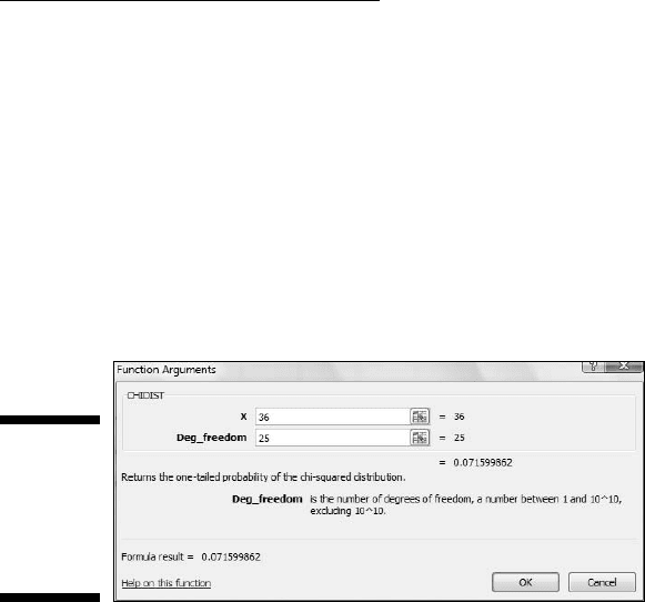
2. From the Statistical Functions menu, select CHIDIST to open the

Function Arguments dialog box for CHIDIST. (See Figure 10-6.)

Figure 10-6:

The

Function

Arguments

dialog box

for CHIDIST.

3. In the Function Arguments dialog box, type the appropriate values for

the arguments.

In the X box, I typed the calculated chi-square value. For this example,

that value is 36.

In the Deg_freedom box, I typed the degrees of freedom. The degrees

of freedom for this example is 25 (26 – 1). After typing the df, the dialog

box shows the one-tailed probability of obtaining at least this value of

chi-square if H

is true.

4. Click OK to close the dialog box and put the answer in the selected cell.

The value in the dialog box in Figure 10-6 is greater than .05, so the decision

is to not reject H

. (Can you conclude that the process is within acceptable

limits of variability? See the nearby sidebar “A point to ponder.”)

CHIINV

CHIINV is the flip side of CHIDIST. You supply a probability and df, and

CHIINV tells you the corresponding value of chi-square. If you want to know

16 454060-ch10.indd 18316 454060-ch10.indd 183 4/21/09 7:29:24 PM4/21/09 7:29:24 PM

184

Part III: Drawing Conclusions from Data

the value you have to exceed in order to reject H

in the preceding example,

follow these steps:

1. Select a cell to store the result.

2. From the Statistical Functions menu, select CHIINV and click OK to

open the Function Arguments dialog box for CHIINV. (See Figure 10-7.)

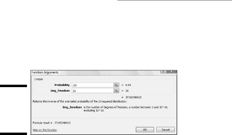
Figure 10-7:

The

Function

Arguments

dialog box

for CHIINV.

3. In the Function Arguments dialog box, enter the appropriate values

for the arguments.

In the Probability box, I typed .05, the probability I’m interested in for

this example.

In the Deg_freedom box, I typed the degrees of freedom. The value for

degrees of freedom in this example is 25 (26 – 1). After I typed the df,

the dialog box shows the value (37.65248) that cuts off the upper 5 per-

cent of the area in this chi-square distribution.

4. Click OK to close the dialog box and put the answer in the selected cell.

As the dialog box in Figure 10-7 shows, the calculated value (36) didn’t miss

the cutoff value by much. A miss is still a miss (to paraphrase “As Time Goes

By”), and you cannot reject H

16 454060-ch10.indd 18416 454060-ch10.indd 184 4/21/09 7:29:24 PM4/21/09 7:29:24 PM

185

Chapter 10: One-Sample Hypothesis Testing

A point to ponder

Retrace the preceding example. FarKlempt

Robotics wants to show that its manufactur-

ing process is within acceptable limits of vari-

ability. The null hypothesis, in effect, says the

process is acceptable. The data do not pres-

ent evidence for rejecting H

. The value of the

test statistic just misses the critical value. Does

that mean the manufacturing process is within

acceptable limits?

Statistics are an aid to common sense, not

a substitute. If the data are just barely within

acceptability, that should set off alarms.

Usually, you try to reject H

. This is a rare

case when not rejecting H

is more desir-

able, because nonrejection implies something

positive — the manufacturing process is work-

ing properly. Can you still use hypothesis testing

techniques in this situation?

Yes, you can — with a notable change. Rather

than a small value of α, like .05, you choose

a large value, like .20. This stacks the deck

against not rejecting H

— small values of the

test statistic can lead to rejection. If α is .20 in

this example, the critical value is 30.6752. (Use

CHINV to verify that.) Because the obtained

value, 36, is higher than this critical value the

decision with this α is to reject H

Using a high α is not often done. When the

desired outcome is to not reject H

, I strongly

advise it.

16 454060-ch10.indd 18516 454060-ch10.indd 185 4/21/09 7:29:24 PM4/21/09 7:29:24 PM

186

Part III: Drawing Conclusions from Data

16 454060-ch10.indd 18616 454060-ch10.indd 186 4/21/09 7:29:24 PM4/21/09 7:29:24 PM

Chapter 11

Two-Sample Hypothesis Testing

In This Chapter

▶ Testing differences between means of two samples

▶ Testing means of paired samples

▶ Testing hypotheses about variances

n business, in education, and in scientific research the need often arises

to compare one sample with another. Sometimes the samples are inde-

pendent, sometimes they’re matched in some way. Each sample comes from

a different population. The objective is to decide whether or not the popula-

tions they come from are different from one another.

Usually, this involves tests of hypotheses about population means. You can

also test hypotheses about population variances. In this chapter, I show you

how to carry out these tests. I also discuss useful worksheet functions and

data analysis tools that help you get the job done.

Hypotheses Built for Two

As in the one-sample case (Chapter 10), hypothesis testing with two samples

starts with a null hypothesis (H

) and an alternative hypothesis (H

). The null

hypothesis specifies that any differences you see between the two samples

are due strictly to chance. The alternative hypothesis says, in effect, that any

differences you see are real and not due to chance.

It’s possible to have a one-tailed test, in which the alternative hypothesis

specifies the direction of the difference between the two means, or a two-

tailed test in which the alternative hypothesis does not specify the direction

of the difference.

17 454060-ch11.indd 18717 454060-ch11.indd 187 4/21/09 7:30:20 PM4/21/09 7:30:20 PM

188

Part III: Drawing Conclusions from Data

For a one-tailed test, the hypotheses look like this:

: μ

- μ

= 0

: μ

- μ

> 0

or like this:

: μ

- μ

= 0

: μ

- μ

< 0

For a two-tailed test, the hypotheses are:

: μ

- μ

= 0

: μ

- μ

≠ 0

The zero in these hypotheses is the typical case. It’s possible, however, to test

for any value — just substitute that value for zero.

To carry out the test, you first set α, the probability of a Type I error that

you’re willing to live with (see Chapter 9). Then you calculate the mean and

standard deviation of each sample, subtract one mean from the other, and

use a formula to convert the result into a test statistic. Compare the test sta-

tistic to a sampling distribution of test statistics. If it’s in the rejection region

that α specifies (see Chapter 10), reject H

. If not, don’t reject H

Sampling Distributions Revisited

In Chapter 9, I introduce the idea of a sampling distribution — a distribution

of all possible values of a statistic for a particular sample size. In that chap-

ter, I describe the sampling distribution of the mean. In Chapter 10, I show its

connection with one-sample hypothesis testing.

For this type of hypothesis testing, another sampling distribution is neces-

sary. This one is the sampling distribution of the difference between means.

The sampling distribution of the difference between means is the distribution

of all possible values of differences between pairs of sample means with the

sample sizes held constant from pair to pair. (Yes, that’s a mouthful.) Held

constant from pair to pair means that the first sample in the pair always has the

same size, and the second sample in the pair always has the same size. The

two sample sizes are not necessarily equal.

17 454060-ch11.indd 18817 454060-ch11.indd 188 4/21/09 7:30:20 PM4/21/09 7:30:20 PM