Velten K. Mathematical Modeling and Simulation: Introduction for Scientists and Engineers

Подождите немного. Документ загружается.

2.1 Elementary Statistics 55

S =

{

x ∈ R|0 ≤ x < 15

}

of this example indeed involves an inﬁnite number of

continuously distributed possible results between 0 and 15 min. In this case, the

following formula can be used [19]:

Proposition 2.1.2 (Relative frequency approximation) Assume that a given

procedure is repeated n times, and let f

(A) denote the relative frequency with

which an event A occurs. Then,

P(A) = lim

n→∞

(A) (2.8)

This means that if we, for example, want to approximate the probability of bus

waiting times between 0 and 2 min (i.e. the probability of A = [0, 2[), the following

approximation can be used

P(A) ≈ f

(A) (2.9)

and the quality of this approximation will increase as n is increased.

2.1.2.3 Densities and Distributions

There is another important approach that can be used to compute probabilities,

which is based on an observation that can be made if a random process is repeated

a great number of times. Let X be a continuous random variable with sample

space S ⊂ R, and let us consider two disjunct events [a

, b

], [a

, b

] ⊂ S,thatis,

, b

] ∩[a

, b

] =∅. Then, suppose that X has been observed n ∈ N times, and

that the same number of observations has been made within [a

, b

]and[a

, b

Now assume that b

− a

> b

− a

. Then, we can say that observations near the

interval [a

, b

] are more likely compared to observations near the interval [a

, b

since the same number of observations was made in each of the two intervals

although [a

, b

] is smaller. If m is the number of observations made in each of the

intervals, then this difference can be made precise as follows:

m/n

− a

m/n

− a

(2.10)

In this equation, m/n approximates the probability of either of the two events

, b

]and[a

, b

] in the sense of Proposition 2.1.2. These probabilities are the same

for both events, but a difference is obtained if they are divided by the respective

sizes of the two intervals, which leads to a quantity known as probability density.

Basically, you can expect more observations within intervals of a given size in

regions of the sample space having a high probability density.

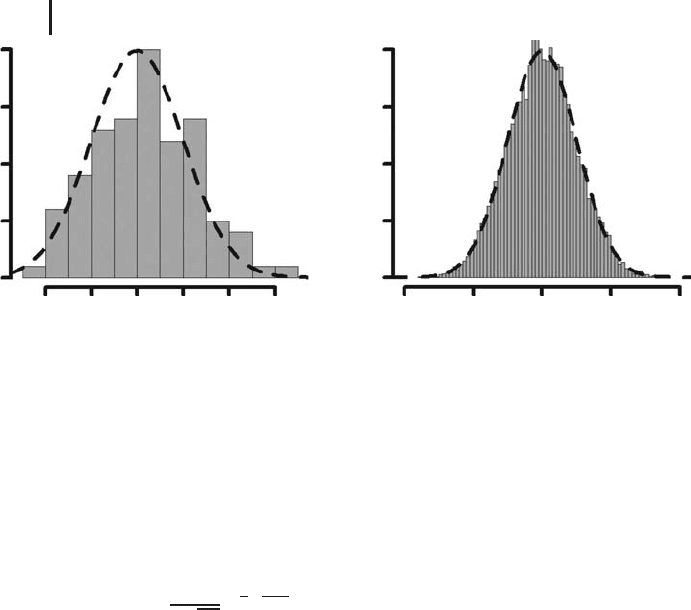
Figure 2.1 shows what happens with the probability density if a random exper-

iment (which is based on a ‘‘normally distributed’’ random variable in this case,

see below) is repeated a great number of times. The ﬁgure is a result of the code

RNumbers.r which you ﬁnd in the book software (Appendix A), and which can

be used to simulate a random experiment (more details on this code will follow

56 2 Phenomenological Models

Probability density

19.8 19.9 20.0 20.1 20.2 20.3 19.6

19.8 20.0 20.2

20.4

(a) (b)

Fig. 2.1 Probability density distributions computed using

RNumbers.r with (a) n = 100 and (b) n = 10 000.

further below). Figure 2.1a and b shows the distribution of the probability density

as a histogram for two cases where the random experiment is repeated (i) 100 and

(ii) 10 000 times. Basically, what can be seen here is that as n is increased, the

probability density approaches the ‘‘bell-shaped’’ function that is indicated by the

dashed line in the ﬁgure, and that can be expressed as:

f (x) =

√

2π

−



x−μ



(2.11)

with μ = 20 and σ = 0.1 in this case. This function is an example of a probability

density function. Probability density functions characterize the random behavior of

a random variable, that is, the behavior of a random variable can be predicted once

we know its probability density function. For example, given a probability densitiy

function f of a random variable X with sample space S ⊂ R, the probability of an

event [a, b] ⊂ S can be computed by the following integral [37]:

P(a ≤ X ≤ b) =



f (t) dt (2.12)

Alternatively, the function

F(x) = P(X ≤ x) =



−∞

f (t) dt (2.13)

is also often used to characterize the behavior of a random variable. It is called

the probability distribution of the random variable. Basically, probability density

functions or probability distributions provide a compact way to describe the

behavior of a random variable. The probability density function in Equation 2.11,

for example, describes the behavior of the random variable based on only two

2.1 Elementary Statistics 57

parameters, μ and σ (more details on this distribution and its parameters will

follow below).

Probability density functions always satisfy f (t) ≥ 0and,ifS = R,



∞

−∞

f (t) dt = 1 (2.14)

that is, the area under the probability density function is always 1 (note that

otherwise Equation 2.12 would make no sense).

2.1.2.4 The Uniform Distribution

The probability density function of the bus waiting time (see above) is

f (x) =

⎧

⎨

⎩

if x ∈ [0, 15[

0 otherwise

(2.15)

that is, in this case the probability density is constant. As discussed above, this

expresses the fact that the same number of observations can be expected within any

interval of a given length within [0, 15]. This makes sense in the bus-waiting-time

example since each particular waiting time between 0 and 15 min is equally likely.

Using Equations 2.12 and 2.15, we can, for example, compute the probability of

waiting times between 3 and 5 min as follows:

P(3 ≤ X

≤ 5) =



f (t) dt =

· (5 −3) =

(2.16)

Equation 2.15 is the probability density function of the uniform distribution,which

is written generally as

f (x) =

⎧

⎨

⎩

b − a

if x ∈ [a, b[

0 otherwise

(2.17)

It is easy to show that the area under this probability density function is 1 as

required by Equation 2.14.

2.1.2.5 The Normal Distribution

Random variables that can be described by the probability density function in

Equation 2.11 are said to have the normal distribution, which is also known as the

Gaussian distribution since it was discovered by C.F. Gauss. In a sense, one can say

that the normal distribution is called normal since it is normal for random processes

to be normally distributed...A great number of random processes in science and

engineering can be described using this distribution. This can be theoretically

justiﬁed based on the central limit theorem, which states that the distribution of a

sum of a large number of independent and identically distributed random variables

can be approximated by the normal distribution (see [37] for details).

58 2 Phenomenological Models

Let us use the notation X ∼ N(μ, σ ) for a random variable X that is normally

distributed with parameters μ and σ (see Equation 2.11; more on these param-

eters will follow in the next section). Remember that a measurement device was

discussed at the beginning of this section, and that we were asking the follow-

ing question: with what probability will the deviation of the measurement value

from the true value be smaller than some speciﬁed value such as 0.1? Assum-

ing that the true value of the measured quantity is 20, and assuming normally

distributed measurement errors (which is typically true due to the central limit

theorem), this question can now be answered using Equations 2.11 and 2.12 as

follows:

P(19.9 ≤ X ≤ 20.1) =



20.1

19.9

√

2π

−



x−μ



dt (2.18)

Unfortunately, this integral cannot be solved in closed form, which means that

numerical methods must be applied to get the result (see Section 3.6.2 for a

general discussion of closed form versus numerical solutions). The simplest way

to compute probabilities of this kind numerically is to use spreadsheet programs

such as Calc. Calc offers a function

NORMDIST that can be used to compute values

either of the probability density function or of the distribution function of the

normal distribution. If F(x) is the distribution function of the normal distribution

(compare Equation 2.13), the above probability can be expressed as

P(19.9 ≤ X ≤ 20.1) = F(20.1) − F(19.9) (2.19)

which can be obtained using Calc as follows:

P(19.9 ≤ X ≤ 20.1) = NORMDIST(20.1;μ;σ ;1) −NORMDIST(19.9;μ;σ ;1)

(2.20)

For example, μ = 20 and σ = 0.1yieldP (19.9 ≤ X ≤ 20.1) ≈ 68, 3%.

We can now explain the background of the code

RNumbers.r that was used

above to motivate probability density functions. This code simulates a normally

distributed random variable based on R’s

rnorm command. The essential part of

this code is the line

out=rnorm(n,mu,sigma)

where rnorm is invoked with the parameters n (number of random numbers to

be generated),

mu and sigma (parameters μ and σ of Equation 2.11). R’s hist

and curve commands are used in RNumbers.r to generate the histogram and the

dashed curve in Figure 2.1, respectively (see the code for details).

2.1.2.6 Expected Value and Standard Deviation

Now it is time to understand the meaning of the parameters of the normal

distribution, μ and σ . Let us go back to the dice example, and let X

be the random

2.1 Elementary Statistics 59

variable expressing the result of the dice as before. Suppose two experiments are

performed:

Experiment 1

The dice is played ﬁve times. The result is: 5, 6, 4, 6, 5.

Experiment 2

The dice is played 10 000 times.

Analyzing Experiment 1 using the methods described in Section 2.1.1, you

will ﬁnd that the average value is

x = 5.2 and the standard deviation is s ≈ 0.84.

Without knowing the exact numbers produced by Experiment 2, it is clear that the

average value and the standard deviation in Experiment 2 will be different from

x = 5.2ands ≈ 0.84. The relatively high numbers in Experiment 1, and hence, the

relatively high average value of

x = 5.2 has been obtained by chance only, and it

is clear that such an average value cannot be obtained in Experiment 2. If you get

a series of relatively high numbers such as the numbers produced in Experiment

1 as a part of the observations in Experiment 2, then it is highly likely that this

will be balanced by a corresponding series of relatively small numbers (assuming

a fair dice, of course). As the sample size increases, the average value of a sample

stabilizes toward a value that is known as the expected value of a random variable X

which is usually denoted as E(X)orμ, and which can be computed as

μ = E(X) =

· 1 +

· 2 +

· 3 +

· 4 +

· 5 +

· 6 = 3.5 (2.21)

in the case of the dice example. This means that we can expect x ≈ 3.5in

Experiment 2. The last formula can be generalized to

μ = E(X) =



i=1

(2.22)

if X is a discrete random variable with possible values x

, ..., x

having probabil-

ities p

, ..., p

. Analogously, the (sample) standard deviation of a sample stabilizes

toward a value that is known as the standard deviation of a random variable X which

is usually denoted as σ , and which can be computed as

σ =









i=1

− μ)

(2.23)

for a discrete random variable. This formula yields σ ≈ 2.92 in the dice example,

that is, we can expect s ≈ 2.92 in Experiment 2. For a continuous random variable

60 2 Phenomenological Models

with probability density function f , the expected value and the standard deviation

can be expressed as follows [37]:

μ =



∞

−∞

t · f (t) dt (2.24)

σ =





∞

−∞

(t − μ)

· f (t) dt (2.25)

As suggested by the notation of the parameters μ and σ of the normal distribution,

it can be shown that these parameters indeed express the expected value and

the standard deviation of a random variable that is distributed according to

Equation 2.11.

2.1.2.7 More on Distributions

Beyond the uniform and normal distributions discussed above, there is a great

number of distribution functions that cannot be discussed in detail here, such as

Student’s t-distribution (which is used e.g. to estimate means of normally distributed

variables) or the gamma distribution (which is used e.g. to describe service times

in queuing theory [38]). Note also that all distribution functions considered so far

were referring to continuous random variables. Of course, the same concept can

also be used for discrete random variables, which leads to discrete distributions.An

important example is the binomial distribution, which refers to binomial random

processes which have only two possible results. Let us denote these two results by

0 and 1. Then, if p is the (ﬁxed) probability of getting a 1 and the experiment is

repeated n times, the distribution function can be written as

F(x) = P(X ≤ x) =

ﬂoor(x)



j=0





(1 −p)

n−j

(2.26)

where ﬂoor(x) returns the highest integer less than or equal to x. See [19, 37] for

more details on the binomial distribution and on other discrete distributions.

2.1.3

Inferential Statistics

While the methods of descriptive statistics are used to describe data, the methods

of inferential statistics, on the other hand, are used to draw inferences from data (it

is as simple as that ...). This is a big topic. Within the scope of this book, we will

have to conﬁne ourselves to a treatment of some basic ideas of statistical testing

that are required in the following chapters. Beyond this, inferential statistics is e.g.

concerned with the estimation of population parameters such as the estimation of

the expected value from data, see [19, 37] for more on that.

2.1 Elementary Statistics 61

2.1.3.1 Is Crop A’s Yield Really Higher?

Suppose the following yields of crops A and B have been measured (in g):

Crop A: 715, 683, 664, 659, 660, 762, 720, 715

Crop B: 684, 655, 657, 531, 638, 601, 611, 651

Thesedataareintheﬁle

crop.csv in the book software (Appendix A). The

average yield is 697.25 for crop A and 628.5 for crop B, and one may therefore be

tempted to say that crop A yields more than crop B. But we need to be careful: can

we be sure that crop A’s yield is really higher, or is it possible that the difference

in the average yields is just a random effect that may be the other way round

in our next experiment? And if the data indeed give us a good reason to believe

that crop A’s yield is higher, can the certainty of such an assertion be quantiﬁed?

Questions of this kind can be answered by the method of statistical hypothesis

testing.

2.1.3.2 Structure of a Hypothesis Test

Statistical hypothesis tests that are performed using software (we do not discuss

the traditional methods here, see [19, 37] for that) usually are conducted along the

following steps:

•

Select the hypothesis to be tested: the null hypothesis,often

abbreviated as H

•

Depending on the test that is performed, you may also have to

select an alternative hypothesis, which is assumed to hold true if

the null hypothesis is rejected as a result of the test. Let H

this alternative hypothesis, or let H

be the negation of H

if no

alternative hypothesis has been speciﬁed.

•

Select the signiﬁcance level α, which is the probability to

erroneously reject a true H

as a result of the test. Make α small

if the consequences of rejecting a true H

are severe. Typical

choices are α = 0.1, α = 0.05, or α = 0.01.

•

Collect appropriate data and then use the computer to perform

an appropriate test using the data. As a result of the test, you will

obtain a pvalue(see below).

•

If p <α, reject H

.Inthiscase,H

is assumed to hold true, and

as well as the test itself are said to be statistically signiﬁcant at

the level α.

Note that in the case of a nonsigniﬁcant test (p ≥ α), nothing can be derived

from the test. In particular – and you need to be careful regarding this point – the

fact that we do not reject H

in this case does not mean that it has been proved by

the test that H

is true. The p value can be deﬁned as follows [37]:

62 2 Phenomenological Models

Deﬁnition 2.1.4 (P value)

The p value (or observed signiﬁcance level) is the smallest level of signiﬁcance at

which H

would be rejected when a speciﬁed test procedure is used on a given

dataset.

In view of the above testing procedure, this deﬁnition may seem somewhat

tautological, so you should note that the ‘‘test procedure’’ in the deﬁnition refers

to the mathematical details of the testing procedure that cannot be discussed here,

see [19, 37].

A hypothesis test may involve two main types of errors: a type I error,wherea

true null hypothesis is rejected, and a type II error, which is the error of failing to

reject a null hypothesis in a situation where the alternative hypothesis is true. As

mentioned above, α is the probability of a type I error, while the probability of a

type II error is usually denoted with β. The inverse probability 1 − β,thatis,the

probability of rejecting a false null hypothesis is called the power of the test [19, 37].

2.1.3.3 The t test

Coming back to the problem discussed in Section 2.1.3.1 above, let X

and X

denote the random variables that have generated the data of crop A and crop B,

respectively, and let μ

and μ

denote the (unknown) expected values of these

random variables. Referring to the general test structure explained in the last

section, let us deﬁne the data of a statistical test as follows:

•

: μ

= μ

•

: μ

>μ

•

α = 0.05

Now a ttestcan be used to get an appropriate p value [37]. This test can be

performed using the program

TTest.r in the book software (Appendix A). If you

run this program as described in Appendix B, it will produce a few lines of text

in which you will read ‘‘p value = 0.00319’’. Since this is smaller compared to the

signiﬁcance level α assumed above, H

is rejected in favor of H

, and hence the

test shows what is usually phrased as follows: ‘‘The yield of crop A is statistically

signiﬁcantly higher (at the 5% level) compared to crop B.’’ Note that this analysis

assumes normally distributed random variables, see [19, 37] for more details.

The main command in

TTest.r that does the computation is t.test,whichis

used here as follows:

t.test(Dataset$x, Dataset$y

,alternative="greater",paired=FALSE)

Dataset$x and Dataset$y are the data of crop A and crop B, respectively, which

TTest.r reads from crop.csv using the read.table command (see TTest.r

for details). alternative can be set to alternative="less" if H

: μ

<μ

used, and to

alternative="two.sided" inthecaseofH

: μ

= μ

. For obvious

2.1 Elementary Statistics 63

reasons, t tests using H

: μ

<μ

or H

: μ

>μ

are also called one-sided t tests,

whereas t tests using H

: μ

= μ

are called two-sided t tests. paired must be set

to true if each of the x values has a unique relationship with one of the y values, for

example, if x is the yield of a fruit tree in year 1 and y is the yield of the same tree in

year 2. This is a paired t test, whereas the above crop yield example – which involves

no unique relationships between the data of crop A and crop B – is called an

independent t test [37]. R’s

t.test command can also be used to perform one-sample

ttestswhere the expected value of a single sample (e.g. the concentration of an

air pollutant) is compared with a single value (e.g. a threshold value for that air

pollutant). Note that t tests can also be accessed using the ‘‘Statistics/Means’’ menu

option in the R Commander.

2.1.3.4 Testing Regression Parameters

A detailed treatment of linear regression will follow below in Section 2.2. At this

point, we just want to explain a statistical test that is related with linear regression.

As we will see below, linear regression involves the estimation of a straight line

y = ax + b or of a hyperplane y = a

+ a

+···+a

from data. Let us focus

on the one-dimensional case, y = ax + b (everything is completely analogous in

higher dimensions). In the applications, it is often important to know whether a

variable y depends on another variable x . In terms of the model y = ax + b,the

question is whether a = 0(i.e.y depends on x)ora = 0(i.e.y does not depend on

x). To answer this question, we can set up a statistical hypothesis test as follows:

•

: a = 0

•

: a = 0

•

α = 0.05

For this test, the line labeled with an ‘‘x’’ in the regression output in Figure 2.2a

reports a p value of p = 0.00318. This is smaller than α = 0.05, and hence we

can say that ‘‘a is statistically signiﬁcantly different from zero (at the 5% level)’’,

which means that y depends statistically signiﬁcantly on x.Inasimilarway,thep

value p = 0.71713 in the line labeled with ‘‘Intercept’’ in the regression output in

Figure 2.2a refers to a test of the null hypothesis H

: b = 0, that is, this p value can

be used to decide whether the intercept of the regression line (i.e. the y value for

x = 0) is signiﬁcantly different from zero. Note that this analysis assumes normally

distributed random variables, and note also that a and b have been used above to

denote the random variables that are generating the slope and the intercept of the

regression line if the regression procedure described in Section 2.2 is performed

based on sample data.

2.1.3.5 Analysis of Variance

The regression test discussed in the previous section can be used to decide

about the dependence of y on x in a situation where x is expressed in terms of

numbers, which is often phrased like this: ‘‘x is at the ratio level of measurement’’

[19]. If x is expressed in terms of names, labels, or categories (the nominal

level of measurement), the same question can be answered using the analysis of

64 2 Phenomenological Models

variance, which is often abbreviated as anova. As an example, suppose that we

want to investigate whether fungicides have an impact on the density of fungal

spores on plants. To answer this question, three experiments with fungicides

A, B, and C and a control experiment with no treatment are performed. Then,

these experiments involve what is called a factor x which has the factor levels

‘‘Fungicide A’’, ‘‘Fungicide B’’, ‘‘Fungicide C’’, and ‘‘No Fungicide’’. At each of

these factor levels, the experiment must be repeated a number of times such

that the expected values of the respective fungal spore densities are sufﬁciently

characterized.

Theresultsofsuchanexperimentcanbefoundintheﬁle

fungicide.csv

in the book software (see Appendix A). Note that the ‘‘Factor’’ column of this

ﬁle corresponds to x, while the ‘‘Value’’ column corresponds to y (it reports the

result of the measurement, i.e. the density of the fungal spores on the plants in

an appropriate unit that we do not need to discuss here). Let X

, X

,andX

denote the random variables that have generated these data, and let μ

, μ

,and

denote the expected values of these random variables. Then, we can set up a

hypothesis test as follows:

•

: μ

= μ

•

:Therearei, j ∈{1, 2, 3, 4} s.t. μ

= μ

•

α = 0.05

Basically, H

says that the factor x does not have any impact on the fungal spore

density y, while the alternative hypothesis H

is the negation of H

. An appropriate

p value for this test can now be computed using the R program

Anova.r in the

book software, which is based on R’s

anova command. If you run this program

as described in Appendix B, it will produce a few lines of text in which you read

‘‘Pr(>F) = 0.000376’’, which means p = 0.000376. Again, the test is signiﬁcant

since we have p <α.Hence,H

can be rejected and we can say that the factor

‘‘fungicide’’ has a statistically signiﬁcant impact on the fungal spore density (again,

at the 5% level).

Note that this analysis assumes random variables that are normally dis-

tributed and which have homogeneous variances (i.e. squared standard devi-

ations), see [19, 37] for more details. The above example is called a one-way

analysis of variance or single-factor analysis of variance since it involves one

factor x only. R’s

anova command and the Anova.r code can also be ap-

plied to situations with several factors x

, ..., x

, which is called a multiway

analysis of variance or multifactor analysis of variance. Note that when you per-

form a multiway analysis of variance using

Anova.r,youwillhavetousea

data ﬁle which provides one column for each of the factors, and one more

column for the measurement value. What we have described so far is also

known as the ﬁxed-effects model of the analysis of variance. Within the gen-

eral scope of the analysis of variance, a great number of different modeling

approaches can be used, for example, random effects models which assume a

hierarchy of different populations whose differences are constrained by the hierar-

chy [39].