Zhang K., Li D. Electromagnetic Theory for Microwaves and Optoelectronics
Подождите немного. Документ загружается.

3.2 Standing Waves in Lossless Lines 121
(3) High Frequency, Small Loss
In the case of relatively high frequency and relatively small loss,
ωL À R, ωC À G.
By retaining only the first-order terms in the binomial expansions of (3.13),
(3.14), and (3.15), we have the following approximations
α ≈
R
2
p
L/C
+
G
p
L/C
2
, β ≈ ω
√
LC, (3.16)
and
Z
C
≈
r
L
C
·
1 + j
µ
G
2ωC
−
R
2ωL
¶¸
. (3.17)
(4) A Lossless Line
In a lossless line, r = 0, G = 0, we have
α = 0, β = ω
√
LC, Z
C
=
r
L
C
. (3.18)
The expressions for the voltage and current become
U(z) = U
+
e
−jβz
+ U
−
e
jβz
, (3.19)
I(z) = I
+
e
−jβz
+ I
−
e
jβz
=
U
+
Z
C
e
−jβz
−
U
−
Z
C
e
jβz
. (3.20)
They become two persistent traveling waves propagating along +z and −z.
The solutions of the voltage and current on a lossless transmission line, (3.19)
and (3.20), are the same as those for the electric and magnetic fields of the
plane wave propagating in the lossless medium.
It can be seen from (3.18) that, in common transmission line which con-
sists of series inductances and shunt capacitances, the phase coefficient β
increases versus frequency. On the contrary, for the transmission line con-
sists of series capacitance and shunt inductances, the phase coefficient β will
decrease versus frequency as shown in problem 3.7. The former represents a
forward wave system and the later represents a backward wave system, see
Chapter 7.
3.2 Standing Waves in Lossless Lines
3.2.1 The Reflection Coefficient, Standing Wave Ratio
and Impedance in a Lossless Line
The relation between the amplitudes of the waves along +z and −z depends
upon the termination of the line. Put a load with an impedance Z
L
at the
122 3. Transmission-Line and Network Theory for Electromagnetic Waves
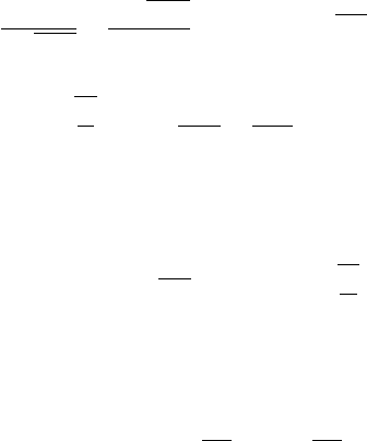
Figure 3.4: Transmission line with load at the terminal z = 0.
end, z = 0, and set the direction from the load to the source as the direction
of +z, see Figure 3.4.
In this sp ecific coordinate system, the term e
jβz
represents the incident
wave and the term e
−jβz
represents the reflected wave. In (3.19), U
−
= U
iL
denotes the amplitude of the voltage of the incident wave at the load, z = 0,
and U
+
= U
rL
denotes the amplitude of the voltage of the reflected wave at
the load. Then the expressions (3.19) and (3.20) b ecome
U(z) = U
iL
e
jβz
+ U
rL
e
−jβz
, (3.21)
I(z) = I
iL
e
−jβz
+ I
rL
e
jβz
=
1
Z
C
¡
U
iL
e
jβz
− U
rL
e
−jβz
¢
. (3.22)
At the load, z = 0, the voltage and the current satisfy Ohm’s law:
Z
L
=
U(0)
I(0)
=
U
iL
+ U
rL
1/Z
C
(U
iL
− U
rL
)
. (3.23)
The reflection coefficient at the load and the load impedance become
Γ
L
= |Γ
L
|e
jφ
L
=
U
rL
U
iL
=
Z
L
− Z
C
Z
L
+ Z
C
, Z
L
= Z
C
1 + Γ
L
1 − Γ
L
. (3.24)
Then the amplitudes of the voltage and current at z become
U(z) = U
iL
¡
e
jβz
+ Γ
L
e
−jβz
¢
, (3.25)
I(z) =
U
iL
Z
C
¡
e
jβz
− Γ
L
e
−jβz
¢
. (3.26)
At any point z on the line, the state of the lossless line can be described
as follows.
(1) The Voltage Reflection Coefficient
The reflection coefficient at the point z is defined as
Γ =
U
r
(z)
U
i
(z)
=
U
rL
e
−jβz
U
iL
e
jβz
= Γ
L
e
−j2βz
= |Γ
L
|e
j(φ
L
−2βz)
= |Γ |e
jφ
, (3.27)
3.2 Standing Waves in Lossless Lines 123
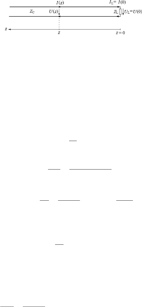
Figure 3.5: Phasor diagram of the voltage and the current on the transmission
line.
where
|Γ | = |Γ
L
|, φ = φ
L
− 2βz. (3.28)
The magnitude of the reflection coefficient is constant along the line, and the
difference between the angles of the reflection coefficients at z and at the load
is 2βz.
At any two points z
1
and z
2
on the line, we have
Γ (z
2
) = Γ (z
1
) e
−j2βl
, (3.29)
where l = z
2
− z
1
.
(2) The Voltage Standing Wave Ratio, VSWR
Substituting Γ
L
in (3.24) into (3.25), we have the distribution of the voltage
along the line:
U(z) = U
iL
e
jβz
h
1 + |Γ |e
j(φ
L
−2βz)
i
, (3.30)
and the magnitude of the voltage becomes
|U(z)| = U
iL
p
1 + |Γ |
2
+ 2|Γ |cos(φ
L
− 2βz). (3.31)
The distribution of the current and its magnitude along the line can be ob-
tained from (3.26):
I(z) =
U
iL
Z
C
e
jβz
h
1 − |Γ |e
j(φ
L
−2βz)
i
, (3.32)
|I(z)| =
U
iL
Z
C
p
1 + |Γ |
2
− 2|Γ |cos(φ
L
− 2βz). (3.33)
124 3. Transmission-Line and Network Theory for Electromagnetic Waves
0.00 .25 .50 .75 1.00 1.25 1.50 1.75 2.00
0.0
.2
.4
.6
.8
1.0
1.2
1.4
1.6
1.8
2.0
*
0.00 .25 .50 .75 1.00 1.25 1.50 1.75 2.00
0.0
.2
.4
.6
.8
1.0
1.2
1.4
1.6
1.8
2.0
*
*
*
*
*
*
(a)
(b)
O
z
Li
)(
U
zU
Li
)(
U
zU
CLi
)(
ZU
zI
CLi
)(
ZU
zI
Li
)(
U
zU
O
z
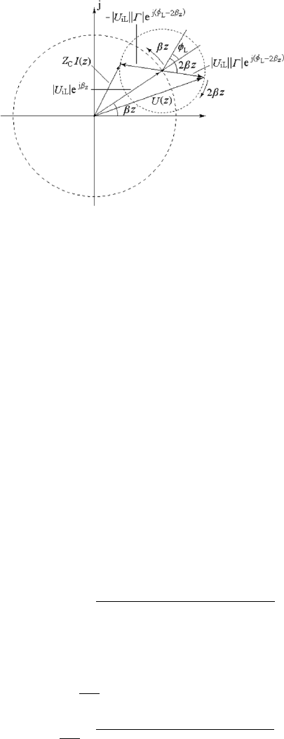
Figure 3.6: Distribution of the voltage and current magnitudes along the
transmission line.
These expressions, (3.30)–(3.33), are similar to those for the reflection
of uniform plane waves, (2.136)–(2.139) and (2.254)–(2.257). The phasor
diagram for (3.30) and (3.31) is shown in Fig. 3.5, and the distribution of the
magnitudes of the voltage and current along the line is shown in Fig. 3.6.
The maximum of the standing wave voltage, U
max
, occurs at φ
L
−
2βz
max
= 2nπ,
U(z
max
) = U
max
= U
iL
(1 + |Γ |), (3.34)
and the minimum, U
min
, occurs at φ
L
− 2βz
min
= (2n + 1)π,
U(z
min
) = U
min
= U
iL
(1 − |Γ |). (3.35)
The current minimum occurs at the point of voltage maximum, and the
current maximum occurs at the point of voltage minimum.
The ratio of U
max
to U
min
is the voltage standing wave ratio, or VSWR
for short, denoted by
ρ = VSWR =
U
max
U
min
=
1 + |Γ |
1 − |Γ |
or |Γ | =
ρ − 1
ρ + 1
. (3.36)
3.2 Standing Waves in Lossless Lines 125
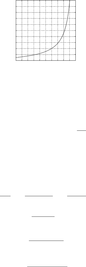
0.0 .1 .2 .3 .4 .5 .6 .7 .8 .9 1.0
0
2
4
6
8
10
12
14
16
18
20
U
|
*
|
(VSWR)
Figure 3.7: Relation between VSWR and the reflection coefficient.
The relation between ρ and |Γ | is plotted in Fig. 3.7. The state of |Γ | = 0
and ρ = 1 corresponds to non-reflection or matching, and the state of |Γ | = 1
and ρ → ∞ corresponds to total reflection.
The angle of the reflection coefficient can be determined by the position
of the voltage minimum of the standing wave, z
min
,
φ
L
= (2n + 1)π + 2βz
min
= (2n + 1)π + 4π
z
min
λ
. (3.37)
The VSWR and the position of the standing-wave minimum are easy to
determine by experiment.
(3) Normalized Impedance and Normalized Admittance
Define the ratio of the complex amplitude of the voltage to the complex
amplitude of the current at any point z on the line as the input impedance
denoted by Z(z). Using (3.25) and (3.26), we have
Z(z) =
U(z)
I(z)
= Z
C
1 + Γ
L
e
−j2βz
1 − Γ
L
e
−j2βz
= Z
C
1 + Γ (z)
1 − Γ (z)
, (3.38)
and
Γ (z) =
Z(z) − Z
C
Z(z) + Z
C
. (3.39)
Substituting (3.24) into (3.38), we have the relation between Z(z) and Z
L
:
Z(z) = Z
C
Z
L
+ jZ
C
tan βz
Z
C
+ jZ
L
tan βz
. (3.40)
The transformation relation between the impedances at two points z
1
and z
2
becomes
Z(z
2
) = Z
C
Z(z
1
) + jZ
C
tan βl
Z
C
+ jZ(z
1
) tan βl
, (3.41)
126 3. Transmission-Line and Network Theory for Electromagnetic Waves
where l = z
2
− z
1
. This is just the same as the impedance transformation
formula in plane waves, refer to Section 2.5.
Similar results hold for the input admittance, load admittance, and char-
acteristic admittance. Let
Y
C
=
1
Z
C
, Y
L
=
1
Z
L
, Y (z) =
1
Z(z)
,
we have
Y (z) = Y
C
1 − Γ (z)
1 + Γ (z)
, (3.42)
Γ (z) =
Y
C
− Y (z)
Y
C
+ Y (z)
, (3.43)
Y (z
2
) = Y
C
Y (z
1
) + jY
C
tan βl
Y
C
+ jY (z
1
) tan βl
. (3.44)
It is convenient for many purposes to introduce the normalized impedance
and the normalized admittance
z = r + jx =
Z
Z
C
, y = g + jb =
Y
Y
C
=
1
z
. (3.45)
Then the above relations become
z =
1 + Γ
1 − Γ
, y =
1 − Γ
1 + Γ
, (3.46)
Γ =
z − 1
z + 1
, Γ =
1 − y
1 + y
, (3.47)
z(z
2
) =
z(z
1
) + j tan βl
1 + jz(z
1
) tan βl
, y(z
2
) =
Y (z
1
) + j tan βl
1 + jY (z
1
) tan βl
. (3.48)
It can be seen from (3.48) that the normalized impedances at two points
on the line with separation λ/2 are equal to each other, and those with
separation λ/4 are reciprocal to each other. This means that at two points
on the line with separation λ/4 the normalized impedance at one point is
equal to the normalized admittance at the other point.
3.2.2 States of a Transmission Line
The state of a transmission line can be described by one of the following four
complex quantities, each including two real quantities:
1. the magnitude and the angle of the complex reflection coefficient,
2. the real and imaginary parts, or the magnitude and the angle of the
normalized impedance,

3.2 Standing Waves in Lossless Lines 127
3. the real and imaginary parts or the magnitude and the angle of the
normalized admittance,
4. the VSWR and the position of the minimum of standing wave voltage.
The different states of the transmission line are as follows.
(1) The Matched Line
Z
L
= Z
C
, Γ
L
= 0.
The reflected wave is zero,
U(z) = U
iL
e
jβz
, I(z) =
U
iL
Z
C
e
jβz
, Z(z) = Z
C
.
It is a traveling wave propagates along the line. The impedance at any point
on the line is equal to the characteristic impedance. The traveling wave on a
matched line is the same as that on an infinitely long line or is similar to a
plane wave propagating in unbounded space.
(2) The Short-Circuit Line
Z
L
= 0, Y
L
→ ∞, Γ
L
= −1.
The amplitude of the reflected wave is equal to that of the incident wave,
U(z) = U
iL
¡
e
jβz
− e
−jβz
¢
= U
m
sin βz, (3.49)
I(z) =
U
iL
Z
C
¡
e
jβz
+ e
−jβz
¢
= −j
U
m
Z
C
cos βz, (3.50)
where U
m
= 2jU
iL
. This is a pure standing wave with the voltage node and
the current maximum at the short-circuit terminal. The impedance at any
point on the line is
Z(z) = jZ
C
tan βz. (3.51)
This result is the same as that for the incidence and reflection of a plane
wave on a perfect conductor plane. This is why a perfect conductor plane is
recognized as a short-circuit plane.
(3) The Open-Circuit Line
Z
L
→ ∞, Y
L
= 0, Γ
L
= 1.
The amplitude of the reflected wave is also equal to that of the incident wave,
U(z) = U
iL
¡
e
jβz
+ e
−jβz
¢
= U
m
cos βz, (3.52)

128 3. Transmission-Line and Network Theory for Electromagnetic Waves
I(z) =
U
iL
Z
C
¡
e
jβz
− e
−jβz
¢
= j
U
m
Z
C
sin βz, (3.53)
where U
m
= 2U
iL
. This is a pure standing wave with the voltage maximum
and the current node at the short circuit terminal. The impedance at any
point on the line is
Z(z) = −jZ
C
cot βz. (3.54)
This result is the same as that for the incidence and reflection of a plane
wave on an open-circuit plane. The standing wave is shifted by a distance of
λ/4 compared with that of the short-circuit line.
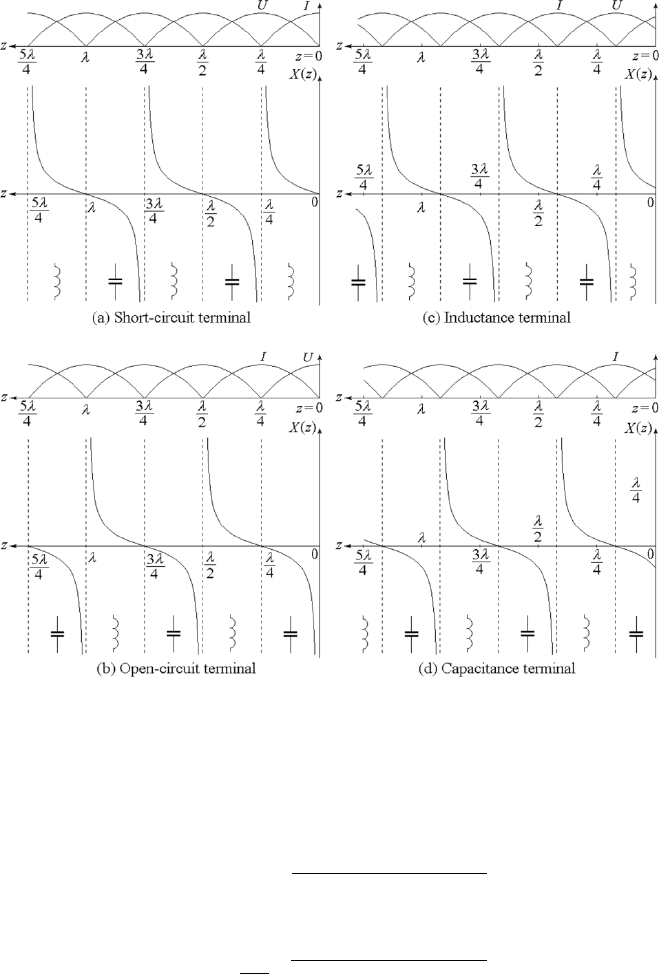
(4) The Reactance-Loaded Line
Z
L
= jX
L
, Γ
L
= e
jφ
L
, |Γ
L
| = 1,
φ
L
= arctan
2X
L
Z
C
X
2
L
− Z
2
C
= arctan
2x
L
x
2
L
− 1
,
where x
L
= X
L
/Z
C
denotes the normalized load reactance. Then, we have
U(z) = U
m
e
jφ
L
/2
cos
µ
βz −
φ
L
2
, (3.55)
I(z) = j
U
m
Z
C
e
jφ
L
/2
sin
µ
βz −
φ
L
2
, (3.56)
Z(z) = −jZ
C
cot
µ
βz −
φ
L
2
. (3.57)
This is also a pure standing wave, but with neither the voltage no de nor the
current node at the terminal, refer to Fig 3.8.
(5) The Resistance-Loaded Line
Z
L
= R
L
, Γ
L
=
R
L
− Z
C
R
L
+ Z
C
=
r
L
− 1
r
L
+ 1
,
where r
L
= R
L
/Z
C
denotes the normalized load resistance. The reflection
coefficient is real. When R
L
< Z
C
, Γ
L
is negative and φ
L
= π, and the
voltage and current along the line become
|U(z)| = U
iL
p
1 + |Γ |
2
− 2|Γ |cos 2βz, (3.58)
|I(z)| =
U
iL
Z
C
p
1 + |Γ |
2
+ 2|Γ |cos 2βz. (3.59)
There is a traveling standing wave or, simply, a standing wave on the line.
The standing-wave voltage minimum and current maximum appear at the
3.2 Standing Waves in Lossless Lines 129
Figure 3.8: Voltage, current and impedance for reactance-loaded line.
load. When R
L
> Z
C
, Γ
L
is positive and φ
L
= 0, and the voltage and
current along the line become
|U(z)| = U
iL
p
1 + |Γ |
2
+ 2|Γ |cos 2βz, (3.60)
|I(z)| =
U
iL
Z
C
p
1 + |Γ |
2
− 2|Γ |cos 2βz. (3.61)
The standing wave voltage-maximum and current minimum appear at the
load.

130 3. Transmission-Line and Network Theory for Electromagnetic Waves
(6) The Arbitrary-Impedance Loaded Line
This is the general case. A traveling standing wave propagates along the line
with neither voltage maximum nor voltage minimum at the load.
The equations for the reflection coefficient and VSWR, the impedance
transformation and the concept of impedance matching for the transmission
line are the same as those for the plane wave and the waves in any guided-wave
system. So transmission-line theory is used to simulate the electromagnetic
waves or even non-electromagnetic waves in any guided-wave system.
3.3 Transmission-Lines Charts
It can be seen from (3.46) that the relation between the two complex variables
z and Γ is a bilinear function. A bilinear function is the transformation of two
sets of orthogonal circle families (the straight line is a special case of circle).
The relation between y and Γ is also a bilinear function, and the relation
between z and y is an inversion transformation. Thus we can construct the
mapping graph of the three complex functions Γ , z, and y, which is known
as a transmission-line chart and is helpful for the calculation of the states of
transmission lines.
For a passive system, the magnitude of Γ cannot be greater than 1, and
the real part of z and y cannot be negative. So the transmission-line chart
must be the mapping of the interior region of a unit circle in polar coordinates
and the positive (right) half plan in the rectangular coordinates.
There are various kinds of transmission-line charts, depending upon the
choice of coordinates.
3.3.1 The Smith Chart
(1) The Smith Impedance Chart
The Smith impedance chart or simply Smith chart is a plot of the complex
function of the normalized impedance z = r + jx on the Γ plane in polar
coordinates. The expression for Γ in terms of z can be written as
Γ = |Γ |e
jφ
= u + jv, z = r + jx.
Then equation (3.46) becomes
r + jx =
1 + (u + jv)
1 − (u + jv)
. (3.62)
This equation may be separated into real and imaginary parts as follows:
r =
1 −
¡
u
2
+ v
2
¢
(1 − u
2
) + v
2
, x =
2v
(1 − u
2
) + v
2
. (3.63)