Enns R.H. Computer Algebra Recipes for Mathematical Physics

Подождите немного. Документ загружается.

158 CHAPTER 4. LINEAR PDES OF PHYSICS

GR2 :=



n=1

⎛

⎜

⎝

4sin(

nπb

)sin(

nπy

) e

(−

nπ(x−a)

)

⎞

⎟

⎠

The parameter values a=0.5, b=0.8, and L= 1 are entered, and the piecewise

Green’s function, G=GL2 for x<aand GR2 for x>a,formed.

a:=0.5: b:=0.8: L:=1:

G:=piecewise(x<a,value(GL2),x>a,value(GR2)):

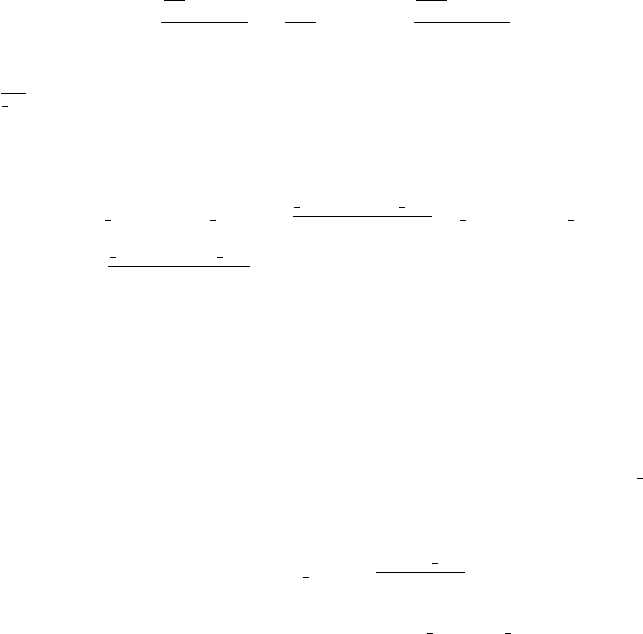
Using contourplot, equipotentials are drawn in cp for G=1/8, 1/4, 1/2, 1, 2, 3

and then superimposed on gr1 and gr2, the result being shown in Fig. 4.10.

The curve closest to the line charge is for G= 3, the furthest for G=1/8.

cp:=contourplot(G,x=-2..2,y=0..L,contours=[1/8,1/4,1/2,

1,2,3],grid=[70,70],color=blue,thickness=2):

display({gr1,gr2,cp},scaling=constrained);

0.5

–0.5 0.5

1.5

Figure 4.10: Equipotentials around line charge between grounded plates.

4.3 Beyond Cartesian Coordinates

Some representative non-Cartesian examples are now presented. Many more

are included in the Supplementary Recipes at the end of the chapter.

4.3.1 Is It Separable?

Alliance. In international politics, the union of two thieves who have

their hands so deeply inserted in each other’s pockets that they can-

not separately plunder a third.

Ambrose Bierce, American author, The Devil’s Dictionary (1881–1906)

The method of separation of variables can be applied to other orthogonal curvi-

linear coordinate systems besides the Cartesian system. I have found that, at

ﬁrst, some students are surprised that the variable separation method works

4.3. BEYOND CARTESIAN COORDINATES 159

at all. After a while, they assume that it always works. It turns out that the

scalar Helmholtz equation, ∇

S +k

S = 0, which is the spatial part of either the

wave or diﬀusion equations with k a constant, is separable [MF53] in 11, and

only 11, 3-dimensional orthogonal curvilinear coordinate systems. Fortunately,

these include spherical polar and cylindrical coordinates, which are the two

most commonly used non-Cartesian systems. An example of a 3-dimensional

coordinate system for which the Helmholtz equation is not separable are the

bispherical coordinates u, v, w, which are related to x, y, z by

x =

a sin u cos v

cosh w − cos u

,y=

a sin u sin v

cosh w − cos u

,z=

a sinh w

cosh w − cos u

. (4.8)

Here a is a scale factor and 0 ≤ u<π,0≤ v ≤ 2 π, −∞ <w<∞.

As the following recipe illustrates, Laplace’s equation is not separable in

bispherical coordinates either, but can be separated into three ODEs by a mod-

iﬁed separation assumption. This is useful, e.g., in determining the potential

outside two spheres of equal diameters, held at diﬀerent potentials, and with

their centers separated by a distance greater than the sphere diameter.

Although, the bispherical system is known (with a =1)toMaple,itis

instructive to tackle the following problem from ﬁrst principles.

(a) Plot the contours in the x-z plane corresponding to holding u and w ﬁxed.

What surfaces are generated if v is constant?

(b) Calculate the scale factors and the Laplacian operator.

the “standard” ansatz, S(u, v, w)=U(u) V (v) W (w).

(d) Show that Laplace’s equation is completely separable if one assumes that

S(u, v, w)=



(cosh w − cos u) U(u) V (v) W (w). Assuming that cosh w>

cos u, identify any special functions which occur in the separated ODEs.

It is assumed that u ≥ 0, u<π, v ≥ 0, v ≤ 2π, and cosh w>cos u.The

coordinate relations are then entered.

restart: with(plots): assume(u>=0,u<Pi,v>=0,v<=2*Pi,

cosh(w)>cos(u)):

x:=a*sin(u)*cos(v)/(cosh(w)-cos(u));

y:=a*sin(u)*sin(v)/(cosh(w)-cos(u));

z:=a*sinh(w)/(cosh(w)-cos(u));

To plot the surfaces corresponding to holding w ﬁxed, let’s form X

+ Y

(Z − a coth w)

+ y

+(z − a coth w)

and simplify the right-hand side.

eq1:=Xˆ2+Yˆ2+(Z-a*coth(w))ˆ2

=simplify(xˆ2+yˆ2+(z-a*coth(w))ˆ2);

eq1 := X

+ Y

+(Z −a coth(w))

sinh(w)

The result is the equation of a sphere of radius a/ sinh w centered at X =0,

An excellent source of electrostatic problems in bispherical and other coordinate systems

is Problems in Mathematical Physics by Lebedev, Skal’skaya, and Uﬂyand (Pergamon, 1966).

160 CHAPTER 4. LINEAR PDES OF PHYSICS

Y =0, and Z = a coth w. Diﬀerent choices of w will generate diﬀerent size

spheres with centers located at diﬀerent Z values.

Similarly, (

√

+ Y

−a cot u)



+ y

−a cot u)

is entered

in eq2 and simpliﬁed.

eq2:=(sqrt(Xˆ2+Yˆ2)-a*cot(u))ˆ2+Zˆ2

=simplify((sqrt(xˆ2+yˆ2)-a*cot(u))ˆ2+zˆ2,symbolic);

eq2 := (

√

+ Y

− a cot(u))

+ Z

sin(u)

To see what type of surface is generated by holding u ﬁxed, let’s set a = 1 and

Y =0 so as to generate plots in the X-Z plane. The unapply command is used

to free up w and u in eq1 and eq2 for plotting purposes.

a:=1: Y:=0: A:=unapply(eq1,w): B:=unapply(eq2,u):

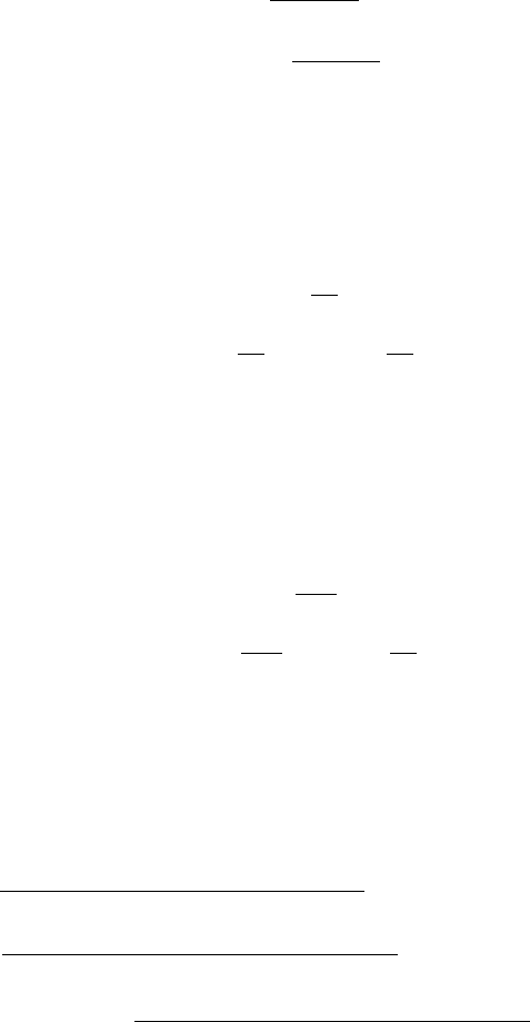
Using A and B and the implicitplot command, representative contours are

drawn for ﬁxed w (solid circles) in gr1 and ﬁxed u (dashed circles) in gr2

gr1:=implicitplot({seq(A(n/2),n=-4..-1),seq(A(n/2),n=1..4)},

X=-5*a..5*a,Z=-5*a..5*a,grid=[70,70],color=red,thickness=2):

gr2:=implicitplot({seq(B(0.2*Pi*n),n=1..4)},X=-5*a..5*a,

Z=-5*a..5*a,grid=[70,70],color=blue,thickness=2,linestyle=2):

and superimposed to produce Fig. 4.11.

display({gr1,gr2},scaling=constrained);

–4

–2 2

Figure 4.11: Contours for ﬁxed w (solid circles) and ﬁxed u (dashed).

The corresponding 3-dimensional surfaces result on rotating the ﬁgure about

the vertical (Z) axis, the circles becoming spheres, hence the name “bispherical”

for the coordinate system. From the deﬁning relations between the bispherical

4.3. BEYOND CARTESIAN COORDINATES 161

and Cartesian systems, one has y/x=sinv/ cos v = tan v, so holding v ﬁxed will

produce half-planes passing through the z-axis.

A functional operator L is created for generating the Laplacian of S(u, v, w)

on specifying the coordinates u, v, w and the scale factors h

, h

L:=(u,v,w,hu,hv,hw)->(diff(hv*hw*diff(S(u,v,w),u)/hu,u)

+ diff(hu*hw*diff(S(u,v,w),v)/hv,v)

+ diff(hu*hv*diff(S(u,v,w),w)/hw,w))/(hu*hv*hw):

An operator H is formed for producing and simplifying the scale factors.

H:=u->simplify(sqrt(diff(x,u)ˆ2+diff(y,u)ˆ2+diff(z,u)ˆ2),

symbolic):

Using H the three scale factors are explicitly calculated.

h[u]:=H(u); h[v]:=H(v); h[w]:=H(w);

cosh(w) − cos(u)

sin(u)

cosh(w) − cos(u)

Then employing L, Laplace’s equation, ∇

S(u, v, w) =0, is generated.

Lap:=L(u,v,w,h[u],h[v],h[w])=0;

Lap :=



cos(u)(

∂

∂u

S(u, v, w))

cosh(w) − cos(u)

sin(u)

(

∂

∂u

S(u, v, w))

(cosh(w) − cos(u))

sin(u)(

∂

∂u

S(u, v, w))

cosh(w) − cos(u)

∂

∂v

S(u, v, w)

(cosh(w) − cos(u)) sin(u)

sin(u)(

∂

∂w

S(u, v, w)) sinh(w)

(cosh(w) − cos(u))

sin(u)(

∂

∂w

S(u, v, w))

cosh(w) − cos(u)



(cosh(w) − cos(u))

/sin(u)=0

An unsuccessful attempt is made to separate Laplace’s equation by assuming

that S(u, v, w)=U(u) V (v) W (w).

pdsolve(Lap,HINT=U(u)*V(v)*W(w));

Warning : Incomplete separation.

(S(u, v, w)=V (v) F1 (u, w)) &where[{

V (v)= c

V (v), ······

The separation is incomplete, an ODE resulting for V (v), but the u and w de-

pendence remaining coupled in a PDE, which is not displayed here in the text.

Supplying the modiﬁed separation assumption as a hint, Laplace’s equation is

now completely separated.

162 CHAPTER 4. LINEAR PDES OF PHYSICS

pdsolve(Lap,HINT=sqrt((cosh(w)-cos(u)))*U(u)*V(v)*W(w),

INTEGRATE);

(S(u, v, w)=



cosh(w) − cos(u) U (u) V (v) W (w)) &where

[{{W (w)=

C5 e

(

√

+ C6 e

(−

√

{V (v)=

C3 e

(

√

+ C4 e

(−

√

{U (u)=

C1 (

cos(2 u) −

)

(1/2 I

√

)

sin(2 u)hypergeom([

√

−

√

], [

cos(2 u)+

)





1 − cos(2 u)+···}}]

W (w)andV (v) are both expressed in terms of exponentials, but U is given in

terms of hypergeometric functions. The hypergeometric function F (a, b; c; z)is

given by the following inﬁnite series [AS72], where Γ is the Gamma function,

F (a, b; c; z)=

Γ(c)

Γ(a)Γ(b)

∞



n=0

Γ(a + n)Γ(b + n)

Γ(c + n)

4.3.2 A Shell Problem, Not a Shell Game

Insurance. An ingenious modern game of chance in which the player

is permitted to enjoy the comfortable conviction that he is beating the

man who keeps the table.

Ambrose Bierce, American author, The Devil’s Dictionary (1881–1906)

In creating physics exams at the freshman level, I often play a bit of a shell

game, presenting problems similar to those that the students have solved for

homework, but in new guises and combinations. The hope is that they really

understand the underlying principles and methods and haven’t merely memo-

rized the solutions to the homework problems. At the senior level, I rely less

on “disguise ” and more on having students explore challenging problems, even

“standard” ones, in some depth. A computer algebra approach is encouraged

as an auxiliary tool. The following recipe, submitted by Ms. I. M. Curious, is

based on a standard problem appearing on an exam given to my senior electro-

magnetic theory class.

A very long circular cylindrical shell of dielectric constant  and inner and

outer radii a and b, respectively, is placed in a previously uniform electric ﬁeld



with the cylinder axis perpendicular to the ﬁeld. The medium inside (r<a)

and outside (r>b) the cylindrical shell has a dielectric constant of unity.

(a) Determine the potential and electric ﬁeld in the three regions.

(b) Taking  =3, a =1, b =2, and E

= 1, plot the equipotentials and electric

ﬁeld vectors in all three regions in a single ﬁgure. Discuss the results and

explore the eﬀect of changing the parameter values.

4.3. BEYOND CARTESIAN COORDINATES 163

In addition to the plots library package, I. M. loads the plottools and VectorCal-

culus packages. Plottools contains the circle command which she will use for

drawing the inner and outer radii of the cylindrical shell. The VectorCalculus

package is needed for the Laplacian and Gradient commands.

restart: with(plots): with(plottools): with(VectorCalculus):

Neglecting end eﬀects, the cylindrical shell is taken to be inﬁnitely long in

the z direction, thus reducing the problem to 2 dimensions in the x-y plane.

Noting the circular symmetry, I. M. introduces the polar coordinates (r, θ)with

x=r cos θ and y = r sin θ, r being measured from the cylinder axis and θ from

the x-axis. Laplace’s equation is entered in polar coordinates and expanded.

pde:=expand(Laplacian(phi(r,theta),’polar’[r,theta]))=0;

pde :=

∂

∂r

φ(r, θ)

∂

∂r

φ(r, θ)) +

∂

∂θ

φ(r, θ)

Using the separation of variables method, a general solution is sought of the

form φ(r, θ)=R(r)Θ(θ). For convenience, I. M. replaces the separation constant

√

that appears on the rhs of sol with the symbol k.

sol:=pdsolve(pde,HINT=R(r)*Theta(theta),INTEGRATE,build);

sol2:=subs(sqrt(_c[1])=k,rhs(sol));

sol2 :=

C3 sin(kθ) C1 r

C3 sin(kθ) C2

+ C4 cos(kθ) C1 r

C4 cos(kθ)

Taking the electric ﬁeld to be in the x direction, I. M. notes that the solution

must have reﬂection symmetry (is unchanged if θ →−θ) around the x axis. So

she removes the sine terms, which are odd functions of θ,fromsol2 .Asr →∞,

the electric ﬁeld must remain uniform and is given by



ˆe

=−(∂φ/∂x)ˆe

so the asymptotic potential is φ= −E

x=−E

r cos θ, the arbitrary constant in

the potential being set equal to zero. This immediately implies that k =1, which

must hold in every region to satisfy the boundary conditions. I. M. substitutes

k = 1 and, without loss of generality, also sets the redundant coeﬃcient

equalto1aswell.

sol3:=subs({_C4=1,k=1},remove(has,sol2,sin));

sol3 := cos(θ)

C1 r +

cos(θ) C2

I. M. labels φ in the regions r<a, a<r<b,andr>bas φ1, φ2, and φ3. An

operator P is formed for relabeling the coeﬃcients

C1and C2foreachφ.

P:=(u,v)->subs({_C1=u,_C2=v},sol3):

For r<a,the1/r term must be removed from φ1 for it to remain ﬁnite at

r =0. SoI.M.formsφ1 by setting v =0 in P and u = A

.Forφ2, she chooses

u = A

, v = B

.Forφ3, she takes u = −E0, in order to match the asymptotic

boundary condition as r →∞,andv = B

164 CHAPTER 4. LINEAR PDES OF PHYSICS

phi1:=P(A[1],0); phi2:=P(A[2],B[2]); phi3:=P(-E0,B[3]);

φ1 := cos(θ) A

φ2 := cos(θ) A

r +

cos(θ) B

φ3:=−cos(θ) E0 r +

cos(θ) B

With A

, A

, B

,andA

unknown, 4 boundary conditions are required. The

potentials φ1=φ2atr = a and φ2=φ3atb for arbitrary θ. The following

operator F is created to match the potentials u and v at a radius r =R.

F:=(u,v,R)-> expand(eval((u=v)/cos(theta),r=R)):

Using F, the above boundary conditions are applied in eq1 and eq2 .

eq1:=F(phi1,phi2,a); eq2:=F(phi2,phi3,b);

eq1 := A

a = A

a +

eq2 := A

b +

= −E0 b +

The radial component of the displacement vector



D = 



E is continuous at the

boundaries, so ∂φ1/∂r =  (∂φ2/∂r)atr = a and  (∂φ2/∂r)=∂φ3/∂r at r = b.

An operator G is created for equating the radial derivative of u and v at a radius

R.UsingG, the two boundary conditions are applied in eq3 and eq4 .

G:=(u,v,R)->expand(eval(diff(u=v,r),r=R)/cos(theta)):

eq3:=G(phi1,epsilon*phi2,a); eq4:=G(epsilon*phi2,phi3,b);

eq3 := A

= εA

−

εB

eq4 := εA

−

εB

= −E0 −

The four equations are solved for the four coeﬃcients and sol4 assigned.

sol4:=solve({eq1,eq2,eq3,eq4},{A[1],A[2],B[2],B[3]});

assign(sol4):

The potentials φ1, φ2, and φ3 are now determined, the coeﬃcients being auto-

matically substituted.

phi1:=phi1; phi2:=simplify(phi2); phi3:=phi3;

φ1:=−

4 cos(θ) ε E0 b

2 εa

− a

+2εb

+ b

− ε

+ b

φ2:=−

2 cos(θ) E0 b

ε + r

+ εa

− a

)

(2 εa

− a

+2εb

+ b

− ε

+ b

) r

φ3:=−cos(θ) E0 r +

cos(θ) E0 b

(−ε

+ b

+ a

− b

)

(2 εa

− a

+2εb

+ b

− ε

+ b

) r

An operator EF is formed for calculating the electric ﬁeld in polar coordinates,

given some potential f.

4.3. BEYOND CARTESIAN COORDINATES 165

EF:=f->-Gradient(f,’polar’[r,theta]):

The electric ﬁeld is then explicitly calculated in each region, but only the ﬁeld

EF1 in region 1 is displayed here.

EF1:=EF(phi1); EF2:=EF(phi2); EF3:=EF(phi3);

EF1 :=

4 cos(θ) ε E0 b

2 εa

− a

+2εb

+ b

− ε

+ ε

−

4sin(θ) ε E0 b

2 εa

− a

+2εb

+ b

− ε

+ ε

The parameter values =3, a=1, b=2, and E

=1 are now entered.

epsilon:=3: a:=1: b:=2: E0:=1:

For plotting purposes, I. M. changes to Cartesian coordinates by entering r =



+ y

,cosθ = x/r and sin θ = y/r.

r:=sqrt(xˆ2+yˆ2): cos(theta):=x/r: sin(theta):=y/r:

The potential V for all three regions is formed with the piecewise command

and the radical expressions simpliﬁed with the radsimp command. The electric

ﬁeld Ef is then calculated from V using the Gradient command and again the

radicals are simpliﬁed.

V:=radsimp(piecewise(r<a,phi1,r<b,phi2,phi3));

Ef:=-radsimp(Gradient(V,[x,y]));

V :=

⎧

⎪

⎨

⎪

⎩

−

4 x



+ y

< 1

−

4(2x

+2y

+1)x

15 (x

+ y

)



+ y

< 2

−

(5 x

+5y

− 8) x

5(x

+ y

)

otherwise

The equipotentials of V are produced in gr1 over the range x=−4..4, y = −4..4

with the contourplot command, 25 contours being requested. I. M. colors the

plot by including filled=true as an option.

gr1:=contourplot(V,x=-4..4,y=-4..4,contours=25,filled=true):

An operator C is formed to plot a thick red circle of radius r, centered at the

origin. Then C is used in gr2 and gr3 to produce circles of radius a and b,

representing the inner and outer radii of the cylindrical shell.

C:=r->circle([0,0],r,color=red,thickness=3):

gr2:=C(a): gr3:=C(b):

The fieldplot command is used in gr4 to plot the electric ﬁeld vectors as

medium sized blue arrows. The density of the arrows is controlled.

gr4:=fieldplot([Ef[1],Ef[2]],x=-4..4,y=-4..4,color=blue,

arrows=MEDIUM,grid=[20,20]):

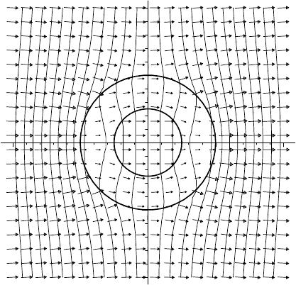
The four graphs are superimposed with the display command, the scaling

being constrained. The resulting picture is shown in Figure 4.12.

display({gr1,gr2,gr3,gr4},scaling=constrained);

166 CHAPTER 4. LINEAR PDES OF PHYSICS

–4

–4 4

Figure 4.12: The electric ﬁeld arrows and equipotentials for a cylindrical dielec-

tric shell inserted in a previously uniform (horizontal) electric ﬁeld.

Referring to the ﬁgure, I. M. notes that the electric ﬁeld for r<ais completely

horizontal and therefore parallel to the asymptotic ﬁeld. The arrows are slightly

shorter however. Quantitatively, the ratio of the electric ﬁeld for r<ato the

asymptotic ﬁeld is A

=4/5. Unlike the situation for a conductor, the

surfaces of the dielectric shell are not equipotentials so the electric ﬁeld vectors

are not perpendicular to the inner and outer surfaces of the shell.

I. M. leaves it to you, the reader, to explore her recipe. For example, you

might take  to be much larger, or alter b with a ﬁxed. She reminds you that

in interpreting any result to remember that the arrows are not ﬁeld lines.

4.3.3 The Little Drummer Boy

Shall I play for you! pa rum pum pum on my drum.

From the Christmas carol, Little Drummer Boy

Little Daniel loves to bang on large pots and pans with a wooden spoon, creat-

ing his own version of music, which to untrained adult ears such as mine sounds

a lot like noise. Here’s a quieter version of “drum playing”.

A large circular drumhead of radius r = a = 1 m has its perimeter ﬁxed.

If the drumhead has an initial shape U(r, θ, 0) = r (1 − r

)sin(2θ)/20 and

is released from rest, determine the shape of the drumhead at arbitrary time

4.3. BEYOND CARTESIAN COORDINATES 167

t>0. Takethewavespeedtobec = 1 m/s. Then, animate the motion of the

drumhead in time steps of 0.1 s over the interval t=0to2s.

After loading the plots and VectorCalculus packages, the wave equation pde

is entered in polar coordinates (r, θ), making use of the Laplacian command.

restart: with(plots): with(VectorCalculus):

pde:=expand(Laplacian(U(r,theta,t),’polar’[r,theta]))

=(1/cˆ2)*diff(U(r,theta,t),t,t);

pde :=

∂

∂r

U (r, θ, t)

∂

∂r

U (r, θ, t)) +

∂

∂θ

U (r, θ, t)

∂

∂t

U (r, θ, t)

Then pde is analytically solved, assuming that U(r, θ, t)=R(r)Θ(θ) T (t).

sol:=pdsolve(pde,HINT=R(r)*Theta(theta)*T(t),INTEGRATE,

build);

sol := U (r, θ, t)=e

(

√

(

√

θ)

C5 C3 C1 BesselJ(

√

− c

√

− c

)

+ e

(

√

(

√

θ)

C5 C3 C2 BesselY(

√

− c

√

− c

)+···

The answer involves exponentials and Bessel functions of the ﬁrst and second

kinds. The separation constants

and c

on the rhs of sol are replaced with

−p

and −c

, and the result simpliﬁed with the symbolic option.

U1:=simplify(subs({_c[2]=-pˆ2,_c[3]=-cˆ2*kˆ2},rhs(sol)),

symbolic);

U1 :=

C5 C3 C1 BesselJ(p, k r) e

((ckt+pθ) I)

+ C5 C3 C2 BesselY(p, k r) e

((ckt+pθ) I)

+ ···

The Bessel functions Y

(kr) of the second kind diverge at r =0, so are removed

from U1 .ThenU2 is converted to trig form and expanded in U3 .

U2:=remove(has,U1,BesselY);

U3:=expand(convert(U2,trig));

U3 :=

C5 C3 C1 BesselJ(p, k r) cos(ckt) cos(pθ)

−

C5 C3 C1 BesselJ(p, k r)sin(ckt)sin(pθ)

C5 C4 C1 BesselJ(p, k r)sin(ckt) cos(pθ) I

C5 C3 C1 BesselJ(p, k r) cos(ckt)sin(pθ) I + ···

The initial transverse velocity of the drumhead is zero, so the sin(ckt)terms

must be removed from U3 . Since the initial shape involves a sine function only,

there can be no cosine terms present in the solution. The cos(pθ) terms are

therefore also removed in U4 and the result then factored.

U4:=factor(remove(has,U3,{sin(c*k*t),cos(p*theta)}));

U4 :=

C1 ( C3 − C4 )( C5 + C6 )sin(pθ) cos(ckt) BesselJ(p, k r)I