Enns R.H. Computer Algebra Recipes for Mathematical Physics

Подождите немного. Документ загружается.

168 CHAPTER 4. LINEAR PDES OF PHYSICS

The solution must vanish at the perimeter, so the Bessel functions J

(kr)must

be zero at r = a.Thus,ka must equal the mth zero of J

,withm =1, 2, ....

The allowed k values are now entered.

k:=BesselJZeros(p,m)/a:

The parameter values a = 1 and c = 1 are given. To match the initial angular

dependence, we must have p= 2, i.e., only the Bessel function J

will be present

in the solution. The radial portion of the initial shape is entered in f.The

form of the Bessel functions is given in g.

a:=1: c:=1: p:=2: f:=r*(1-rˆ2/aˆ2)/20; g:=BesselJ(p,k*r);

f :=

r (−r

+1)

g := BesselJ(2, BesselJZeros(2,m) r)

The messy constants are removed from U4 with the following select command.

U[2,m]:=select(has,U4,{cos,sin,BesselJ});

2,m

:= cos(BesselJZeros(2,m) t)sin(2θ) BesselJ(2, BesselJZeros(2,m) r)

Making use of orthogonality and noting that the weight function for the Bessel

functions is r,themth coeﬃcient is given by A

2,m



frgdr/



dr.

A[2,m]:=int(f*r*g,r=0..a)/int(r*gˆ2,r=0..a):

Theﬁrst4termsoftheseriessolutionU are now displayed in decimal form.

U:=evalf(sum(A[2,m]*U[2,m],m=1..4));

U := 0.04223579864 cos(5.135622302 t)sin(2.θ) BesselJ(2., 5.135622302 r)

+0.002159293112 cos(8.417244140 t)sin(2.θ) BesselJ(2., 8.417244140 r)

+0.005912588156 cos(11.61984117 t)sin(2.θ)BesselJ(2., 11.61984117 r)

+0.001008506062 cos(14.79595178 t)sin(2.θ) BesselJ(2., 14.79595178 r)

For animation purposes, we convert from polar coordinates to Cartesian coordi-

nates, setting r =



+ y

and using the trig identity sin(2 θ)=2 sinθ cos θ =

2 xy/r

. Note that a ﬂoating point evaluation is used in entering the latter so

that the substitution will actually occur. This is necessary because a ﬂoating

point evaluation was used in expressing U.

r:=sqrt(xˆ2+yˆ2): sin(evalf(2*theta)):=2*x*y/rˆ2:

The solution is then expressed as the piecewise function UU =U for r<aand

0forr>a.

UU:=evalf(piecewise(r<a,U,r>a,0)):

To animate UU , a functional operator gr is created to make a 3-dimensional

plot of the drumhead shape on the ith time step, the stepsize being 0.1 s.

gr:=i->plot3d(eval(UU,t=0.1*i),x=-a..a,y=-a..a,

style=patchcontour,shading=zhue):

Then using the sequence command, the proﬁles on 20 consecutive time steps are

displayed. The insequence=true option is included to produce the animation.

display([seq(gr(i),i=1..20)],insequence=true,axes=framed);

If you wish to see the drumhead animation, execute the recipe on your computer,

then click on the computer plot and on the start arrow in the tool bar.

4.3. BEYOND CARTESIAN COORDINATES 169

4.3.4 The Cannon Ball

The sound of a kiss is not so loud as that of a cannon,

but its echo lasts a great deal longer.

Oliver Wendell Holmes Sr., American writer, physician, (1809–94)

In the re-enactment of a Civil war battle, a cannon is ﬁred and a hot spheri-

cal iron cannon ball plunges into an icy lake whose temperature is very close

to freezing (0

◦

C). If the cannon ball has a radius R = 20 cm and is initially

100

◦

C throughout on entering the lake, determine the temperature distribu-

tion inside the cooling cannon ball as a function of time. Plot the temperature

distribution in 1 minute intervals up to 15 minutes. What is the temperature

at the center of the cannon ball 15 minutes after plunging into the lake? For

iron, K/(ρC)=0.185 in cgs units, where K is the thermal conductivity, ρ the

density, and C the speciﬁc heat.

After loading the plots and VectorCalculus packages,

restart: with(plots): with(VectorCalculus):

the heat diﬀusion equation ∇

T =(1/a

)(∂T/∂t), with T the temperature and

≡ K/(ρC), is entered in spherical polar coordinates (r, θ, φ). r is the radial

distance from the center of the cannon ball, θ is the angle that the radial vector

makes with the z-axis, and φ is the angle that the projection of the radial vector

into the x-y plane makes with the x-axis.

pde:=expand(Laplacian(T(r,theta,phi,t),’spherical’))

[r,theta,phi]=diff(T(r,theta,phi,t),t)/aˆ2;

pde :=

∂

∂r

T (r, θ, φ, t))

∂

∂r

T (r, θ, φ, t)) +

cos(θ)(

∂

∂θ

T (r, θ, φ, t))

sin(θ)

∂

∂θ

T (r, θ, φ, t)

∂

∂φ

T (r, θ, φ, t)

sin(θ)

∂

∂t

T (r, θ, φ, t)

Since the initial temperature of the cannon ball is uniform throughout, the so-

lution will have no angular dependence. Assuming that T (r, θ, φ, t)=R(r) F (t),

the heat ﬂow equation pde is analytically solved using the pdsolve command.

sol:=pdsolve(pde,HINT=R(r)*F(t),INTEGRATE,build);

sol := T (r, θ, φ, t)=

C3 e

C1 sinh(

√

C3 e

C2 cosh(

√

The hyperbolic sine (sinh) term remains ﬁnite at the origin (r =0), but the cosh

term diverges to ∞ and must be removed from the rhs of sol.

T1:=remove(has,rhs(sol),cosh);

170 CHAPTER 4. LINEAR PDES OF PHYSICS

T1 :=

C3 e

C1 sinh(

√

The separation constant

is replaced with −k

in T1 and the result simpliﬁed

with the symbolic option.

T2:=simplify(subs(_c[1]=-kˆ2,T1),symbolic);

T2 :=

C3 e

(−a

C1 sin(kr) I

It should be noted that the term sin(kr)/r is ([AS72]) just the zeroth order

spherical Bessel function of the ﬁrst kind.

Making use of the select command,

the coeﬃcient combination

C3 C1 I in T2 is replaced with the symbol A.

T3:=A*select(has,T2,{exp,sin,r});

T3 :=

(−a

sin(kr)

Taking the radius of the cannon ball to be R, the surface of the ball is held at

0 degrees, so sin(kR) = 0, and therefore k = nπ/R,withn =1, 2, ....Entering

this result, the nth normal mode of the temperature is displayed in T4 .

k:=n*Pi/R: T4:=T3;

T4 :=

(−

)

sin(

nπr

)

The initial temperature is 100

◦

throughout the cannon ball. Noting that the

weight function ([AS72]) for the spherical Bessel functions is r

, orthogonality

leads to the following expression for the coeﬃcients:



100 (sin(kr)/r) dr/



(sin(kr)/r)

dr.

A is now calculated, assuming that n is an integer.

A:=int(rˆ2*100*sin(k*r)/r,r=0..R)/int(rˆ2*(sin(k*r)/r)ˆ2,

r=0..R) assuming n::integer;

A :=

200 (−1)

(1+n)

nπ

The formal series representation of the temperature distribution T inside the

cannon ball is now completely determined. Retaining 200 terms in the series,

T has the following structure.

T:=Sum(T4,n=1..200);

T :=

200



n=1

⎛

⎜

⎝

200 (−1)

(1+n)

(−

)

sin(

nπr

)

nπr

⎞

⎟

⎠

The spherical Bessel functions j

of the ﬁrst kind are related to the “ordinary” Bessel

functions by the relation j

(x) ≡



(π/2x)J

n+1/2

(x).

4.3. BEYOND CARTESIAN COORDINATES 171

Taking R =20 and a =

√

0.185, T is now evaluated, but not displayed.

T:=eval(value(T),{R=20,a=sqrt(0.185)}):

An arrow operator gr is formed to plot T at 60 s (1 min) intervals.

gr:=i->plot(eval(T,t=i*60),r=0..20,numpoints=1000):

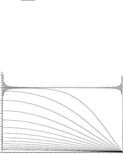
Using gr and the sequence command, the temperature T is displayed as a

function of radius r in Figure 4.13 at t = 0 (top curve), t = 1 min (next lowest

curve), etc, to t= 15 minutes (bottom curve).

display(seq(gr(i),i=0..15),labels=["r","T"]);

100

Figure 4.13: Time evolution of the temperature T inside the cannon ball.

The “ringing” in the initial temperature distribution is, of course, the Gibb’s

phenomenon due to the initial step function temperature proﬁle. Taking the

limit of T as r → 0, the temperature at the center of the sphere at 15 minutes,

or 900 seconds, is calculated and found to be about 3.3

◦

Tcenter:=eval(limit(T,r=0),t=900);

Tcenter := 3.287377363

4.3.5 Variation on a Split-sphere Potential

Would you convey my compliments to the purist who reads your

proofs and tell him or her ... that when I split an inﬁnitive, God damn

it, I split it so it will stay split.

Raymond Chandler, American writer of detective ﬁction, (1888–1959)

The following recipe is based on a simple variation of a standard problem in

electrostatics. The objective is to completely determine the potential V inside

and outside a hollow sphere of unit radius with a speciﬁed piecewise potential

on the spherical surface. With θ measured from the positive z-axis (point-

ing vertically upwards), the spherical surface between θ = 0 and 45

◦

has the

172 CHAPTER 4. LINEAR PDES OF PHYSICS

constant potential V0, the intermediate section between 45

◦

and 135

◦

has a

variable potential given by

√

2 cos(θ) V0 , and the lower portion between 135

◦

and 180

◦

held at −V0 . Keeping the ﬁrst 6 non-zero terms in V and taking

V0 = 1, plot the equipotentials corresponding to V =0.8, 0.6, ..., −0.6, −0.8.

After loading the necessary library packages, Laplace’s equation is entered in

spherical coordinates, the origin taken at the center of the sphere. By symmetry,

V must be independent of the azimuthal

angle φ, i.e., V = V (r, θ).

restart: with(plots): with(VectorCalculus):

pde:=expand(Laplacian(V(r,theta),’spherical’

[r,theta,phi]))=0;

pde :=

∂

∂r

V(r, θ))

∂

∂r

V(r, θ)) +

cos(θ)(

∂

∂θ

V(r, θ))

sin(θ)

∂

∂θ

V(r, θ)

Then pde is analytically solved, assuming that V (r, θ)=R(r)Θ(θ), the result

involving Legendre functions.

V:=rhs(pdsolve(pde,HINT=R(r)*Theta(theta),INTEGRATE,build));

V :=

C3 LegendreP(−

√

1+4 c

,cos(θ)) C1 r

(1/2

√

1+4 c

)

√

+ ···

The separation constant c

is replaced in V with −1/4+(n +1/2)

and the

result simpliﬁed with the symbolic option and then expanded.

V:=expand(simplify(subs(_c[1]=-1/4+(n+1/2)ˆ2,V),symbolic));

V :=

C3 LegendreP(n, cos(θ)) C1 r

C3 LegendreP(n, cos(θ)) C2

+ C4 LegendreQ(n, cos(θ)) C1 r

C4 LegendreQ(n, cos(θ)) C2

V is expressed in terms of the Legendre functions of the ﬁrst (P

(cos θ)) and

second (Q

(cos θ)) kinds. The Q

diverge at the end points of the θ range and

must be rejected. The redundant constant

C3 in the P

terms is set equal to

1and

C1and C2 are replaced with the symbols A and B.

V:=subs({LegendreQ(n,cos(theta))=0,_C3=1,_C1=A,_C2=B},V);

V := LegendreP(n, cos(θ)) Ar

LegendreP(n, cos(θ)) B

For the inside (r<1) solution Vin, we set B =0 in V so that Vin doesn’t

diverge at the origin. For r>1, we take A= 0 so that Vout → 0asr →∞.

Vin:=subs(B=0,V); Vout:=subs(A=0,V);

Vin := LegendreP(n, cos(θ)) Ar

The angle between the projection of the radius vector into the x-y (horizontal) plane and

the x-axis.

4.3. BEYOND CARTESIAN COORDINATES 173

Vout :=

LegendreP(n, cos(θ)) B

Setting u=cosθ, the angular distributions in each region are entered.

f1:=-V0: f2:=sqrt(2)*u*V0: f3:=V0:

Making use of orthogonality of the P

(u),thecoeﬃcientsintheseriesrepre-

sentation of the solution are evaluated using A

=((2 n +1)/2)



−1

(u) du.

An operator AA is introduced to evaluate the coeﬃcients for a given n value.

AA:=n->((2*n+1)/2)*(int(f1*LegendreP(n,u),u=-1..-1/sqrt(2))

+int(f2*LegendreP(n,u),u=-1/sqrt(2)..1/sqrt(2))

+int(f3*LegendreP(n,u),u=1/sqrt(2)..1)):

Then, employing AA(n), the inside and outside solutions are determined, the

series being terminated at n= 12.

VIN:=sum(eval(Vin,A=AA(n)),n=0..12);

VIN :=

cos(θ)V0 r −

LegendreP(3, cos(θ))V0 r

−

128

LegendreP(5, cos(θ))V0 r

2048

LegendreP(7, cos(θ))V0 r

323

8192

LegendreP(9, cos(θ))V0 r

−

1219

65536

LegendreP(11, cos(θ))V0 r

VOUT:=sum(eval(Vout,B=AA(n)),n=0..12);

VOUT :=

cos(θ)V0

−

LegendreP(3, cos(θ))V0

+ ···

The equipotentials will now be plotted in the x-z plane, by setting r =

√

+ z

and cos θ =z/r. We also set V 0=1.

r:=sqrt(xˆ2+zˆ2): cos(theta):=z/r: V0:=1.0:

A piecewise potential function VPW is formed with V = VIN for r<1and

VOUT for r>1.

VPW:=piecewise(r<1,VIN,r>1,VOUT):

Loading the plottools package, a blue circle of radius 1 centered on the origin

is produced in c to represent the spherical surface (a circle in 2 dimensions).

with(plottools): c:=circle([0,0],1,color=blue,thickness=2):

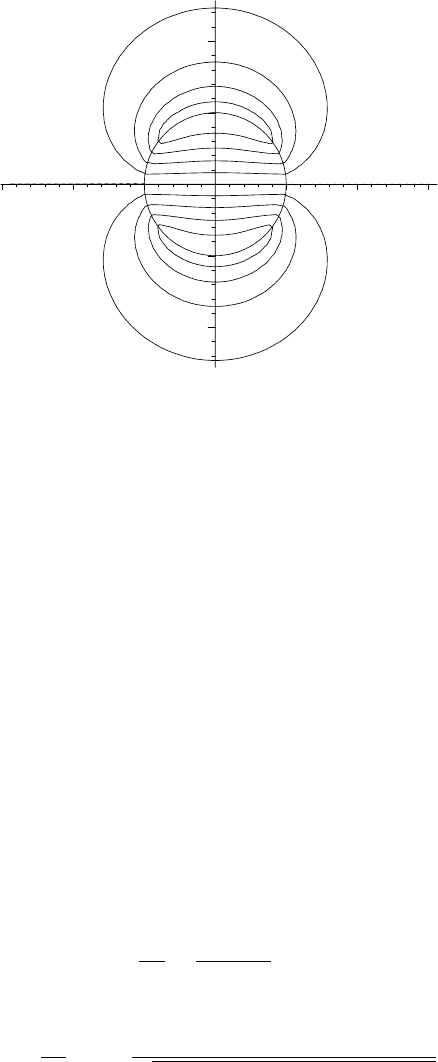
The contourplot command is used in cp to plot the requested equipotentials.

cp:=contourplot(VPW,x=-3..3,z=-4..4,contours=

[seq(0.8-0.2*i,i=0..8)],grid=[60,60],thickness=2,color=red):

The graphs c and cp are now displayed together with constrained scaling,

display({c,cp},scaling=constrained);

the resulting picture being shown in Figure 4.14.

174 CHAPTER 4. LINEAR PDES OF PHYSICS

–2

–3

Figure 4.14: Equipotentials for the split-sphere in the x-z plane.

The 3-dimensional equipotential surfaces are obtained by mentally rotating the

picture about the z-axis. The recipe is easily adjusted to handle other variations

on the angular distribution and can even be modiﬁed to handle cylindrical

geometry.

4.3.6 Another Poisson Recipe

Every man is a potential genius until he does something.

Sir Herbert Beerbohm Tree, English actor-manager, (1853–1917)

In magnetostatics, the vector potential



R )atapoint



R, associated with

a current density



J in free space, satisﬁes the vector Poisson equation, [Gri99]

∇



A = −µ



J, (4.9)

where µ

is the permeability of free space. Equation (4.9) is three scalar Poisson

equations, one for each Cartesian component, e.g., ∇

=−µ

. In any other

curvilinear coordinate system, the unit vectors are functions of position. Thus,

e.g., in spherical polar coordinates it is not true that ∇

=−µ

Assuming that



J → 0 at inﬁnity, the solution of Eq. (4.9) is given by,



R )=

4 π





)



R −



, (4.10)

again representing three 3-dimensional integrals, e.g.,

(x, y, z)=

4 π



) dx



(x − x

)

+(y − y

)

+(z − z

)

4.3. BEYOND CARTESIAN COORDINATES 175

If you want to calculate the integrals in Equation (4.10) in other curvilinear

coordinates, you must ﬁrst express



J in terms of its Cartesian components.

Once



A is determined, the magnetic ﬁeld is then given by



B = ∇×



A.Asa

representative example, consider the following magnetostatic problem.

A uniformly charged solid sphere of radius a carries a total charge Q and

is spinning with angular velocity ω about the vertical z-axis. Determine the

magnetic vector potential



A inside and outside the sphere and then calculate

the magnetic ﬁeld



B in both regions. Plot



B/(µ

Qω)fora=1.

Taking the origin at the sphere’s center, we let



R (r, θ, φ) be the location

of the “observation” point P inside or outside the sphere and



R1(r1 , θ1, φ1)

be the location of a current density “source” point P

inside the sphere. The

polar angles θ and θ1 are measured from the z-axis and the azimuthal angles φ

and φ1 from the projection of the radius vector into the (horizontal) x-y plane

with the x-axis. To ensure a later simpliﬁcation, it is assumed that r>0.

restart: with(plots): with(VectorCalculus): assume(r>0):

Since the charge is uniformly distributed in the sphere, the charge density ρ is

equal to the total charge Q divided by the volume 4 πa

/3 of the sphere. At a

radial distance r1 and angle θ1withthez-axis, the source point P

has a linear

velocity r1 sin(θ1) ω. So the current density magnitude J is equal to ρ times

the linear velocity, the entered form of ρ being automatically substituted. The

corresponding vector



J points in the

φ direction for every P

rho:=Q/((4*Pi*aˆ3)/3); J:=rho*r1*sin(theta1)*omega;

ρ :=

3 Q

4 πa

J :=

Q r1 sin(θ1) ω

πa

Without loss of generality, let’s take the observation point P to be in the x-z

plane, so that φ=0. The position vector



R of P is now entered, being expressed

in terms of the Cartesian unit vectors along the x and z axes.

R:=<r*sin(theta),0,r*cos(theta)>;

R := r sin(θ)e

+ r cos(θ)e

The position vector



R1 of the source point P

is also entered.

R1:=<r1*sin(theta1)*cos(phi1),r1*sin(theta1)*sin(phi1),

r1*cos(theta1)>;

R1 := r1 sin(θ1) cos(φ1) e

+ r1 sin(θ1) sin(φ1) e

+ r1 cos(θ1) e

To calculate



A, let’s ﬁrst evaluate 1/(|



R−



R1|)=1/



(



R −



R1) · (



R −



R1). This

is done in f using the DotProduct command, the result then being simpliﬁed

with the symbolic option.

f:=simplify(1/sqrt(DotProduct(R-R1,R-R1)),symbolic);

f :=



− 2 r sin(θ) r1 sin(θ1) cos(φ1) + r1

− 2 r cos(θ) r1 cos(θ1)

We could attempt to evaluate the integral in



A directly, but it is more instructive

to Taylor expand f about a speciﬁed value of r1, out to some given order, and

176 CHAPTER 4. LINEAR PDES OF PHYSICS

see what the various orders contribute to the overall answer. This approach

is equivalent to the multipole expansion discussed in standard electromagnetic

texts such as Griﬃths [Gri99]. So, a functional operator T is formed to Taylor

expand f to order n about a speciﬁed point r1 =d.Theconvert( ,polynom)

command is included to remove the order of term which would otherwise appear.

T:=(n,d)->convert(taylor(f,r1=d,n),polynom):

The current density vector can be resolved into the Cartesian components

= J sin(φ1), J

= J cos(φ1), and J

= 0. At the observation point (cho-

sen in the x-z plane), the J

contribution to



A will add up to zero, but the J

contribution will not. But since, our choice of observation point in the x-z plane

was arbitrary and there is complete rotational symmetry about the z-axis, the

resultant component J

will yield the φ component of



A. A functional operator

A is created to perform the volume integration in (4.10) using J

and the Taylor

expansion of f and taking spherical polar coordinates. The volume element is

sin(θ1) dθ1 dφ1 dr1 . The angular coordinate θ1 ranges from 0 to π, while

φ1 varies from 0 to 2π. The order n, the radial distance d about which Taylor

expansion is taking place, and the lower and upper limits, d1andd2, of the r1

integration must be speciﬁed. Again the result is simpliﬁed.

A:=(n,d,d1,d2)->simplify((mu[0]/(4*Pi))*int(int(int(T(n,d)

*J*cos(phi1)*r1ˆ2*sin(theta1),theta1=0..Pi),r1=d1..d2),

phi1=0..2*Pi),symbolic):

First, let’s take the observation point P to be outside the sphere, i.e., r>a.

Since r1 ≤ a,thenr1 /r < 1 and we can Taylor expand f about r1 =d=0. The

limits of the r1 integration are d1=0 and d2=a. Making uses of the operator

A with the above arguments, the vector potential is evaluated in Out to order

n= 1, 2, and 3 and the result assigned.

Out:=seq(A||n=A(n,0,0,a),n=1..3); assign(Out):

Out := A1 =0, A2 =

sin(θ) a

Qω

πr

, A3 =

sin(θ) a

Qω

πr

For n = 1, the so-called monopole contribution A1 to the vector potential is 0,

a well-known general result. For n = 2, there is a non-zero dipole contribution

A2 .Forn = 3 (and higher), there is no additional contribution to the vector

potential, indicating that outside the sphere the vector potential (and hence,

the magnetic ﬁeld) is that of a “pure” magnetic dipole. The vector potential

Aout outside the sphere is now expressed in spherical polar coordinates, having

only a φ component.

Aout:=VectorField(<0,0,A2>,’spherical’[r,theta,phi]);

Aout :=

sin(θ) a

Qω

πr

Now, consider P to be inside the sphere, i.e., r<a.Forr1 <r, we can again

Taylor expand f about r1 = 0, the integration being from r1 =0 to r. But for

r1 >r, f is Taylor expanded about r1 =∞,ther1 integration being from r to

a. Adding the two contributions,



A inside the sphere is calculated for n =1, 2,

4.3. BEYOND CARTESIAN COORDINATES 177

and 3. No further contribution occurs for higher n values.

In:=seq(AA||n=A(n,0,0,r)+A(n,infinity,r,a),n=1..3);

assign(In):

In := AA1 =0, AA2 =

sin(θ) Qωr

πa

AA3 =

sin(θ) Qωr

πa

−

Qωrsin(θ)(−a

+ r

)

πa

In terms of spherical polar coordinates, the vector potential Ain inside the

sphere takes the following form.

Ain:=VectorField(<0,0,AA||3>,’spherical’[r,theta,phi]);

Ain := (

sin(θ) Qωr

πa

−

Qωrsin(θ)(−a

+ r

)

πa

) e

Using Curl, the magnetic ﬁeld is calculated outside and inside the sphere.

Bout:=Curl(Aout); Bin:=simplify(Curl(Ain));

Bout :=

Qωcos(θ)

sin(θ) µ

Qω

Bin := −

cos(θ) µ

Qω(3 r

− 5 a

)

πa

sin(θ) µ

Qω(6 r

− 5 a

)

πa

To plot



B/(µ

Qω), the MapToBasis command is used to convert the normalized

magnetic ﬁeld to Cartesian coordinates.

F:=u->MapToBasis(u/(mu[0]*Q*omega),’cartesian’[x,y,z]):

Taking a = 1, we will plot the magnetic ﬁeld in the x-z plane. To accomplish

this, let’s set r =

√

+ z

and form an operator G to evaluate the magnetic

ﬁeld for y =0.

a:=1: r:=sqrt(xˆ2+zˆ2): G:=B->simplify(eval(F(B),y=0)):

The magnetic ﬁeld inside and outside the sphere then takes the following forms,

expressed in Cartesian coordinates.

Bin2:=G(Bin); Bout2:=G(Bout);

Bin2 :=

3 xz

20 π

−

6 x

+3z

− 5

20 π

Bout2 :=

3 zx

20 (x

+ z

)

(5/2)

−

−2 z

+ x

20 (x

+ z

)

(5/2)

The complete magnetic ﬁeld



B is formed with the piecewise operator PW, taking

the nth component of Bin2 and Bout2 for r<aand r>a, respectively.

PW:=n->piecewise(r<a,Bin2[n],r>a,Bout2[n]):

The x and z components of



B are obtained by taking n=1 and 3 in PW.

B[1]:=PW(1): B[3]:=PW(3):

In c, a blue circle of radius a is plotted to represent the spherical surface.

c:=plot(a,theta=0..2*Pi,coords=polar,color=blue,thickness=2):

The fieldplot command is used in fp to plot the magnetic ﬁeld as thick red

arrows, the grid density being taken to be 10 × 10.