Francoise J.-P., Naber G.L., Tsun T.S. (editors) Encyclopedia of Mathematical Physics

Подождите немного. Документ загружается.

(ii) The following observations may clarify the

role of assumptions in the compactness theorem:

(1) a sequence of integral currents (T

) with M(T

)

uniformly bounded – but not M(@T

) – may

converge to any current with finite mass, not

necessarily a rectifiable one.

(2) A sequence of rectifiable currents (T

) with

rectifiable boundaries and M(T

), M(@T

) uniformly

bounded may converge to any normal current,

not necessarily a rectifiable one. Examples of both

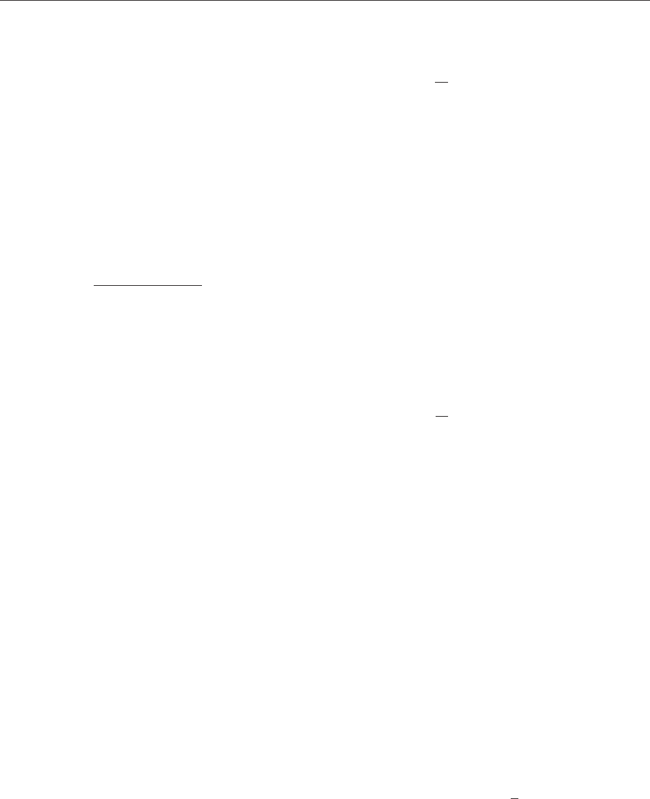
situations are described in Figure 5.

Application to the Plateau Problem

The compactness result for integral currents implies

the existence of currents with minimal mass: if  is

the boundary of an integral k-current in R

,1 k 

n, then there exists a current T of minimal mass

among those that satisfy @T =.

The proof of this existence result is a typical

example of the direct method: let m be the infimum

of M(T) among all integral currents with boundary

, and let (T

) be a minimizing sequence (i.e., a

sequence of integral currents with boundary  such

that M(T

) converges to m). Since M(T

) is bounded

and M(@T

) = M() is constant, we can apply the

compactness theorem for integral currents and

extract a subsequence of (T

) that converges to an

integral current T. By the continuity of the boundary

operator, @T = lim @T

=, and by the semiconti-

nuity of the mass M (T)  lim M(T

) = m (cf. [14]).

Thus, T is the desired minimal current.

Remarks

(i) Every integral (k  1)-current  with null

boundary and compact support in R

is the boundary

of an integral current, and therefore is an admissible

datum for the previous existence result.

(ii) A mass-minimizing integral current T is more

regular than a general integral current. For k = n  1,

there exists a closed singular set S with dim

(S) 

k  7suchthatT agrees with a smooth surface in the

complement of S and of the support of the boundary.

In particular, T is smooth away from the boundary

for n  7. For general k, it can only be proved

that dim

(S)  k  2 Both results are optimal: in

 R

, the minimal 7-current with boundary  :=

{jxj= jyj= 1} – a product of two 3-spheres – is the

cone T := {jxj= jyj1}, and is singular at the origin.

In R

 R

, the minimal 2-current with boundary

 := {x = 0, jyj= 1} [ {y = 0, jxj= 1} – a union of

two disjoint circles – is the union of the disks

{x = 0, jyj1} [ {y = 0, jxj1}, and is singular at

the origin.

(iii) In certain cases, the mass-minimizing current

T may not agree with the solution of the Plateau

problem suggested by intuiti on. The first reason is

that currents do not include nonorientable surfaces,

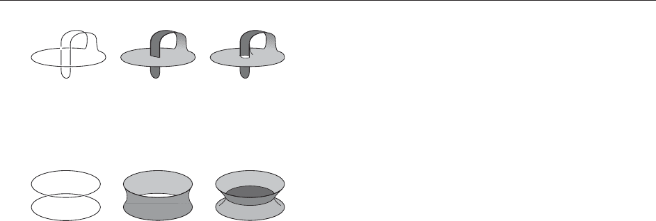
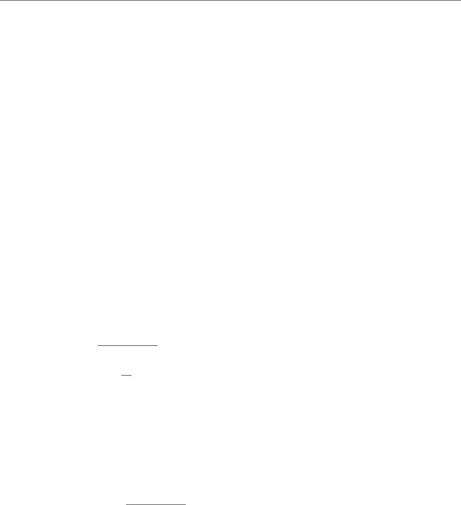
which sometimes may be more convenient (Figure 6).

Another reason is that the mass of an integral

current T associated with a k-rectifiable set E does

not agree with the measure H

(E) – called size of T

– because multiplicity must be taken into account,

and for certain  the mass-minimizing current may

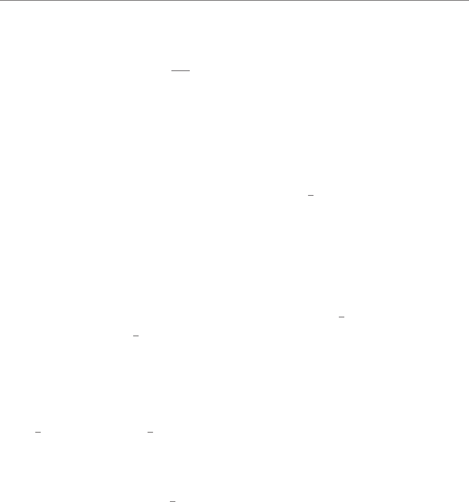
be not size-minimizing (Figure 7). Unfortunately,

proving the existence of size-minimizing currents is

much more complicated, due to lack of suitable

compactness theorems.

(iv) For k = 2, the classical approach to the

Plateau problem consists in parametrizing surfaces

in R

by maps f from a given two-dimensional

domain D into R

, and looking for minimizers of

the area functional

ﬃﬃﬃﬃﬃﬃﬃﬃﬃﬃﬃﬃﬃﬃﬃﬃﬃﬃﬃﬃﬃﬃﬃﬃﬃ

detðrf



rf Þ

:= e·1

:= [E

, e, 1/j]

1/j

Length

= 1/j

1/j

′

:= [E

, e, 1]

′′

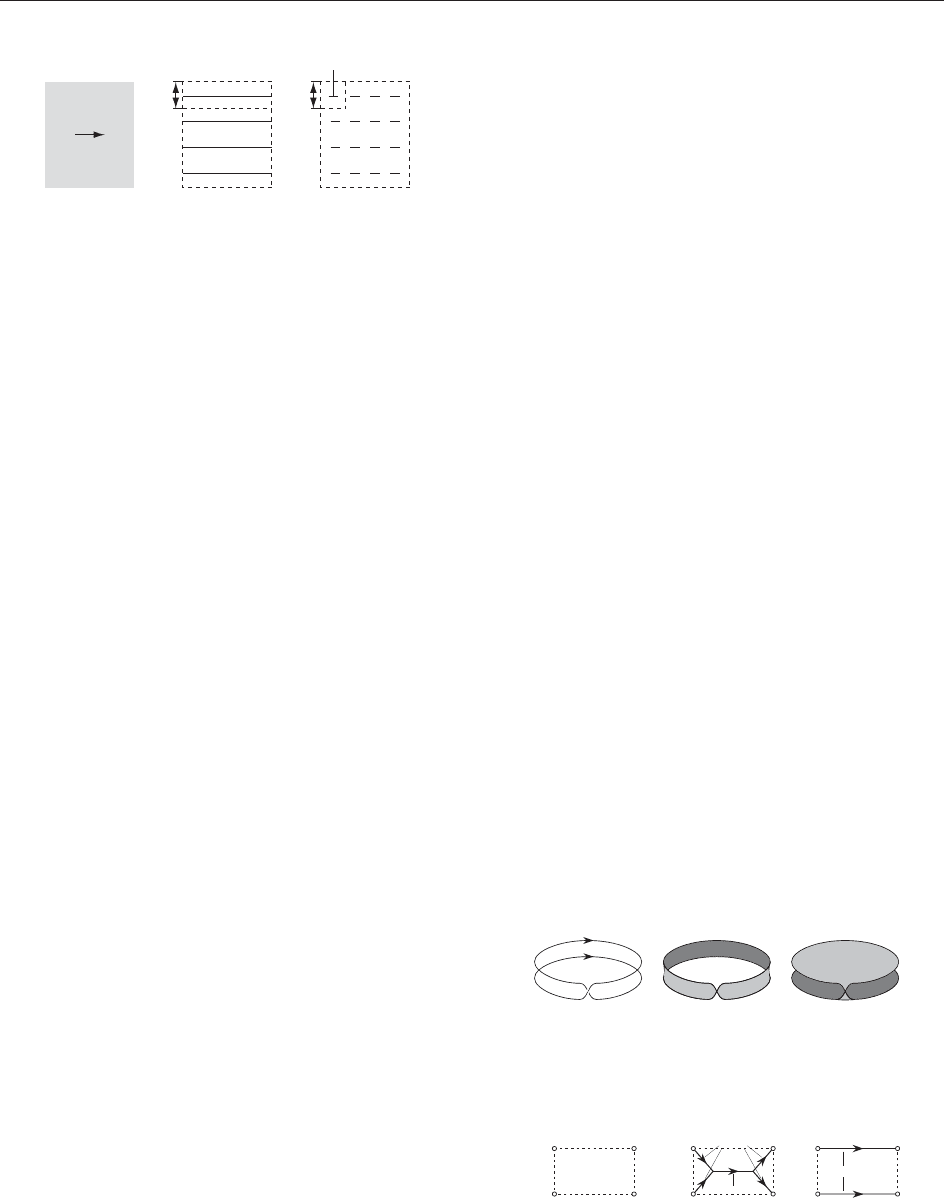
Figure 5 T is the normal 1-current on R

associated with the

vectorfield equal to the unit vector e on the unit square , and

equal to 0 outside. T

are the rectifiable currents associated with

the sets E

(middle) and the constant multiplicity 1=j, and then

M(T

) = 1, M(@T

) = 2. T

are the integral currents associated

with the sets E

(left) and the constant multiplicity 1, and then

M(T

) = 1, M(@T

) = 2j

. Both (T

) and (T

) converge to T.

–1

Γ T

' ′

θ = 2

= 1

θ = 1

′

Figure 7 The boundary  is a 0-current associated with four

oriented points. The size (length) of T is smaller than that of T

However, @T = implies that the multiplicity of T must be 2 on

the central segment and 1 on the others; thus the mass of T is

larger than its size. The size-minimizing current with boundary 

is T, while the mass-minimizing one is T

ΓΣ

Σ′

Figure 6 The surface with minimal area spanning the

(oriented) curve  is the Mo

bius strip . However,  is not

orientable, and cannot be viewed as a current. The mass-

minimizing current with boundary  is 

526 Geometric Measure Theory

(recall the area formula, discussed earlier) under the

constraint f (@D) =. In this framework, the choice

of the domain D prescribes the topological type of

admissible surfaces, and therefore the minimizer

may differ substantially from the mass-minimizing

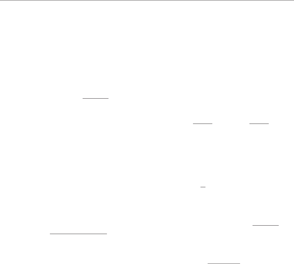
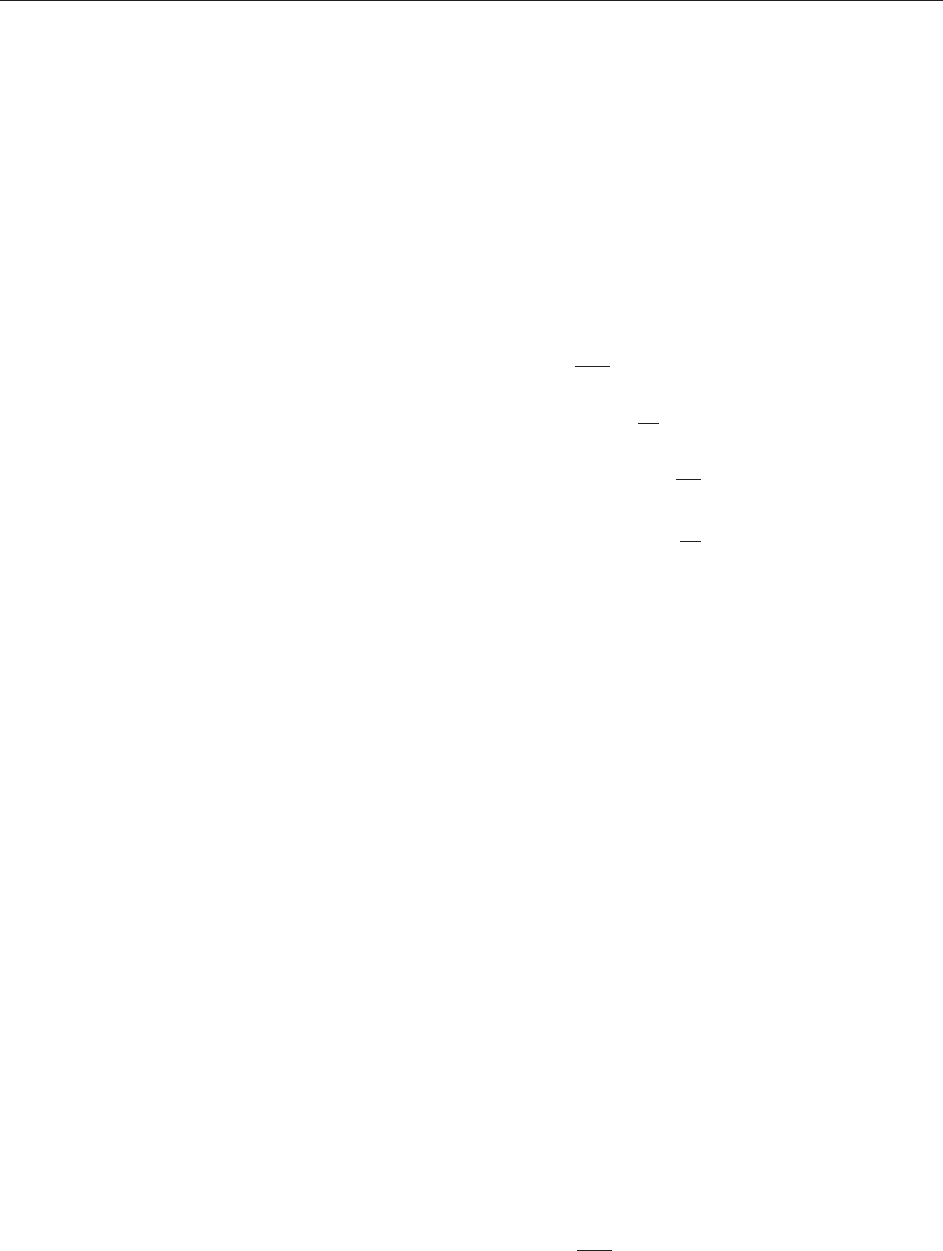
current with boundary  (Figure 8).

(v) For some modeling problems, for instance,

those related to soap films and soap bubbles, currents

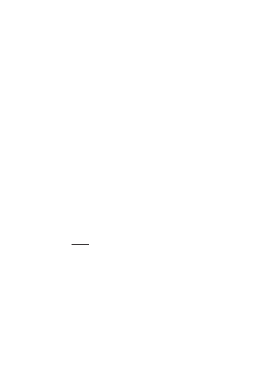
do not provide the right framework (Figure 9). A

possible alternative are integral varifolds (cf. Almgren

2001). However, it should be pointed out that this

framework does not allow for ‘‘easy’’ application of

the direct method, and the existence of minimal

varifolds is in general quite difficult to prove.

Miscellaneous Results and Useful Tools

(i) An important issue, related to the use of currents

for solving variational problems, concerns the extent

to which integral currents can be approximated by

regular objects. For many reasons, the ‘‘right’’ regular

class to consider are not smooth surfaces, but integral

polyhedral currents, that is, linear combinations with

integral coefficients of oriented simplexes. The follow-

ing approximation theorem holds: for every integral

current T in R

there exists a sequence of integral

polyhedral currents (T

)suchthat

! T;@T

! @T

MðT

Þ!MðTÞ; Mð@T

Þ!Mð@TÞ

The proof is based on a quite useful tool, called

polyhedral deformation.

(ii) Many geometric operations for surfaces have an

equivalent for currents. For instance, it is possible to

define the image of a current in R

via a smooth proper

map f : R

. Indeed, with every k-form ! on R

is canonically associated a k-form f

! on R

,called

pullback of ! according to f. The adjoint of the

pullback is an operator, called push-forward, that

takes every k-current T in R

into a k-current f

T in

.IfT is the rectifiable current associated with a

rectifiable set E and a multiplicity , the push-forward

T is the rectifiable current associated with f (E ) – and

a multiplicity 

(y) which is computed by adding up

with the right sign all (x)withx 2 f

1

(y). As one

might expect, the boundary of the push-forward is the

push-forward of the boundary.

(iii) In genera l, it is not possible to give a meaning

to the intersection of two currents, and not even of

a current and a smooth surface. However, it is

possible to define the intersection of a normal

k-current T and a level surfa ce f

1

(y) of a smooth

map f : R

(with k  h  n) for almost every

y, resulting in a current T

with the expected

dimension h  k. This operation is called slicing.

(iv) When working with currents, a quite useful

notion is that of flat norm:

FðTÞ :¼ inf fMðRÞþMðSÞ: T ¼ R þ @Sg

where T and R are k-currents, and S is a (k þ 1)-

current. The relevance of this notion lies in the fact

that a sequence (T

) that converges with respect to

the flat norm converges also in the dual topology,

and the converse holds if the masses M(T

) and

M(@T

) are unifor mly bounded. Hence, the flat

norm metrizes the dual topology of currents (at

least on sets of currents where the mass and the

mass of the boundary are bounded).

Since F(T) can be explicitly estimated from above, it

can be quite useful in proving that a sequence of

currents converges to a certain limit. Finally, the flat

norm gives a (geometrically significant) measure of how

far apart two currents are: for instance, given the 0-

currents 

and 

(the Dirac masses at x and y,

respectively), then F(

 

) is exactly the distance

between x and y.

See also: Free Interfaces and Free Discontinuities:

Variational Problems; -Convergence and

Homogenization; Geometric Phases; Image Processing:

Mathematics; Minimal Submanifolds; Mirror Symmetry:

A Geometric Survey; Moduli Spaces: An Introduction.

Further Reading

Almgren FJ Jr. (2001) Plateau’s Problem: An Invitation to

Varifold Geometry, Revised Edition, Student Mathematical

Library, vol. 13. Providence: American Mathematical Society.

Falconer KJ (2003) Fractal Geometry. Mathematical Foundations

and Applications, 2nd edn. Hoboken, NJ: Wiley.

Federer H (1969) Geometric Measure Theory, Grundlehren der

mathematischen Wissenschaften, vol. 153. Berlin: Springer.

(Reprinted in the series Classics in Mathematics. Springer, Berlin,

1996).

ΓΣ

Σ′

Figure 8 The surface  minimizes the area among surfaces

parametrized by the disk with boundary . The mass-minimizing

current 

can only be parametrized by a disk with a handle.

Note that  is a singular surface, while 

is not.

Σ′

Figure 9 Two possible soap films spanning the wire : unlike

, 

cannot be viewed as a current with multiplicity 1 and

boundary .

Geometric Measure Theory 527

Federer H and Fleming WH (1960) Normal and integral currents.

Annals of Mathematics 72: 458–520.

Mattila P (1995) Geometry of Sets and Measures in Euclidean

Spaces, Fractals and Rectifiability, Cambridge Studies in

Advanced Mathematics, vol. 44. Cambridge: Cambridge

University Press.

Morgan F (2000) Geometric Measure Theory. A Beginner’s

Guide, 3rd edn. San Diego: Academic Press.

Simon L (1983) Lectures on Geometric Measure Theory.

Proceedings of the Centre for Mathematical Analysis, 3.

Australian National University, Centre for Mathematical

Analysis, Canberra 1983.

Geometric Phases

PLe´ vay, Budapest University of Technology and

Economics, Budapest, Hungary

Introduction

We invite the reader to perform the following simple

experiment. Put your arm out in front of you keeping

your thumb pointing up perpendicular to your arm.

Move your arm up over your head, then bring it down

to your side, and at last bring the arm back in front of

you again. In this experiment an object (your thumb)

was taken along a closed path traced by another object

(your arm) in a way that a simple local law of transport

was applied. In this case the local law consisted of two

ingredients: (1) preserve the orthogonality of your

thumb with respect to your arm and (2) do not rotate

the thumb about its instantaneous axis (i.e., your arm).

Performing the experiment in this way, you will

manage to avoid rotations of your thumb locally;

however, in the end you will experience a rotation of



globally.

The experiment above can be regarded as the

archetypical example of the phenomenon called

anholonomy by physicists and holonomy by math-

ematicians. In this article, we consider the manifes-

tation of this phenomenon in the realm of quantum

theory. The objects to be transported along closed

paths in suitable manifolds will be wave functions

representing quantum systems. After applying local

laws dictated by inputs coming from physics, one

ends up with a new wave function that has picked

up a complex phase factor. Phases of this kind are

called geometric phases, with the famous Berry

phase being a special case.

The Space of Rays

Let us consider a quantum system with physical

states represented by elements j i of some Hilbert

space H with scalar product hji:HH ! C. For

simplicity, we assume that H is finite dimensional,

H’C

nþ1

with n  1. The infinite-dimensional case

can be studied by taking the inductive limit n !1.

Let us denote the complex amplitudes characterizing

the state j i by Z



,  = 0, 1, ..., n. For a normalized

state,

k k

¼h j i













¼ 1 ½1

where summation over repeated indices is understood,

indices raised and lowered by 



and 



,respectively,

and the overbar refers to complex conjugation. A

normalized state lies on the unit sphere S’S

2nþ1

nþ1

. Two nonzero states j i and j’i are equivalent,

j ij’i, iff they are related as j i= j’i for some

nonzero complex number . For equivalent states,

physically meaningful quantities such as

h jAj i

h j i

;

jh j’ij

k k

k’k

½2

(mean value of a physical quantity represented by a

Hermitian operator A, transition probability from a

physical state represented by j i to one represented

by j ’i) are invariant. Hence, the real space of states

representing the physical states of a quantum system

unambiguously is the set of equivalence classes P

H= . P is called the ‘‘space of rays.’’ For H’C

nþ1

we have P’CP

, where CP

is the n-dimensional

complex projective space. For normalized states, j i

and j’i are equivalent iff j i= j’i, where jj= 1,

that is,  2 U(1). Thus, two normalized states are

equivalent iff they differ merely in a complex phase.

It is well known that S can be regarded as the total

space of a principal bundle over P with structure

group U(1). This means that we have the projection

 : j i2SH!j ih j2P ½3

where the rank-1 projector j ih j represents the

equivalence class of j i. Since we will use this bundle

frequently in this article, we call it 

(the meaning of

the subscript 1 will be clarified later). Then, we have



: Uð1Þ,!S!



P½4

For Z

6¼ 0 the space of rays P can be given local

coordinates

 Z

; j ¼ 1; ...; n ½5

528 Geometric Phases

The w

are inhomogeneous coordinates for CP

the coordinate patch U

defined by the con dition

6¼ 0.

P is a compact complex manifold with a natural

Riemannian metric g. This metric g is induced from

the scalar product on H. Let us consider the

construction of g by using the physical input

provided by the invariance of the transition prob-

ability of [1]. For this we define a distance between

j ih j and j’ih’j in P as follows:

cos

ðð ;’Þ=2Þ

jh j’ij

k k

k’k

½6

This definition makes sense since, due to the

Cauchy–Schwartz inequality, the right-hand side of

[6] is non-negative and 1. It is equal to 1 iff j i is

a nonzero complex multiple of j’i, that is, iff they

define the same point in P. Hence in this case,

( , ’) = 0 as expected.

Suppose now that j i and j’i are separa ted by an

infinitesimal distance ds  ( , ’). Putting this into

the definition [6], using the local coordinates w

[5] for j i and w

þ dw

for j’i after expanding both

sides using Taylor series, one gets

¼ 4g



; j;



k ¼ 1; 2; ...; n ½7

where





ð1 þ



Þ





ð1 þ



½8

with dw



 d



. The line element [7] defines the

Fubini–Study metric for P.

The Pancharatnam Connection

Having defined the basic entity, the space of rays P,

and the principal U(1) bundle 

, now we define a

connection giving rise to a local law of parallel

transport. This approach gives rise to a very general

definition of the geometric phase. In the math ema-

tical literature, the connection defined below is

called the ‘‘canonical connection’’ on the principal

bundle. However, since the motivation is coming

from physics, we are going to rediscover this

construction using merely physical information

provided by quantum theory alone.

The information needed is an adaptation of Pan-

charatnam’s study of polarized light to quantum

mechanics. Let us consider two normalized states j i

and j’i. When these states belong to the same ray, then

we have j i= e

i

j’i for some phase factor e

i

; hence,

the phase difference between them can be defined to be

just . How to define the phase difference between j i

and j’i (not orthogonal) when these states belong to

different rays? To compare the phases of

nonorthogonal states belonging to different rays,

Pancharatnam employed the following simple rule:

two states are ‘‘in phase’’ iff their interference is

maximal. In order to find the state j’ie

i

j’

i from

the ray spanned by the representative j’

i which is ‘‘in

phase’’ with j i,wehavetofinda modulo 2 for

which the interference term in

jj þ e

i

’

¼ 2ð1 þ Reðe

i

h j’

iÞÞ ½9

is maximal. Obviously the interference is maxi mal

iff e

i

h j’

i is a real positive number, that is,

i

h’

j i

jh’

j ij

; j’i¼j’

h’

j i

jh’

j ij

½10

Hence for the state j’i ‘‘in phase’’ with j i, one has

h j’i¼jh j’

ij 2 R

½11

When such j i and j’ij þ d i are infinitesi-

mally separated, from [11] it follows that

Imh jd i¼



 d





¼ 0 ½12

where



(1 þ



) = 1 due to normal-

ization. Writing Z

jZ

i

using [5], one obtains

Imh jd i¼d þ A ¼ 0; A  Im



1 þ



½13

In order to clarify the meaning of the 1-form A,

notice that the choice

i

ﬃﬃﬃﬃﬃﬃﬃﬃﬃﬃﬃﬃﬃﬃﬃﬃﬃﬃﬃﬃﬃ

1 þ





½14

defines a local section of the bundle 

. In terms of

this section, the state j i can be expressed as

j i¼



¼jZ

i



¼ e

i

i½15

For a path w

(t) lying entirely in U

P,

j (t)i= e

i(t)

(t) i defines a path in S with a

(t) satisfying the equation

 þ A = 0. For a closed

path C, the equation above defines a (generically)

open path  projecting onto C by the projection .

It must be clear by now that the process described is

the one of parallel transports with respect to a

connection with a connection 1-form !. The pull-

back of ! with respect to the local section in [14] is

the 1-form (U(1) gauge field) A in [13]. The curve 

corresponding to j (t)i is the horizontal lift of C in

P. The U(1) phase

i½C

 e

i

½16

Geometric Phases 529

is the holonomy of the connection. We call this

connection the ‘‘Pancharatnam connection,’’ and its

holonomy for a closed path in the space of rays is

the geometric phase acquired by the wave function.

Now the question of fundamental importance is:

how to realize closed paths in P physically? This

question is addressed in the following sections.

Quantum Jumps

We have seen that physical states of a quantum

system are represented by the space of rays P and

normalized states used as representatives for

such states form the total space S of a principal

U(1) bundle 

over P. Moreover, in the previous

section we have realized that the physical

notions of transition probability, and quantum

interference naturally lead t o the introduction of a

Riemannian metric g and an abelian U(1) gauge

field A living on P.

An interesting result based on the connection

between g and A concerns a nice geometric descrip-

tion of a special type of quantum evolution consist-

ing of a sequence of ‘‘quantum jumps.’’

Consider two nonorthogonal rays jAihAj and

jBihBj in P. Le t us suppose that the system’s

normalized wave function initially is jAi2S, and

measure by the ‘‘polarizer’’ jBihBj. Then the result of

this filtering measurement is jBihBjAi, or after

projecting back to the set of normalized states we

have the ‘‘quantum jump’’

jAi!jBi

hBjAi

jhBjAij

½17

Now we have the following theorem:

Theorem The [17] jump can be recovered by

parallel transporting the normalized state jAi

according to the Pancharatnam connection along

the shortest geodesic (with respect to the [8] metric),

connecting jAihAj and jBihBj in P.

Let us now consider a cyclic series of filtering

measurements with projectors jA

ihA

j, a = 1, 2, ...,

N þ 1, where jA

ihA

j= jA

Nþ1

ihA

Nþ1

j. Prepare the

system in the state jA

i2S, and then subject it to

the sequence of filtering measurements. Then

according to the theorem, the phase

i

ihA

N1

ihA

jhA

ihA

N1

ihA

½18

picked up by the state is equal to the one obtained

by parallel transporting jA

i along a geodesic

polygon consisting of the shorte r arcs connecting

the projectors jA

ihA

j and jA

aþ1

ihA

aþ1

j with

a = 1, 2, ..., N. It is important to realize that this

filtering measurement process is not a unitary one;

hence, unitarity is not essential for the geometric

phase to appear.

In this section we have managed to obtain closed

paths in the form of geodesic polygons in P via the

physical process of subjecting the initial stat e jA

i to

a sequence of filtering measurements. It is clear that

for any type of evolution, the geodesics of the

Fubini-study metric play a fundamental role since

any smooth closed curve in P can be approximated

by geodesic polygons.

Nonunitary evolution provided by the quantum

measuring process is only half of the story. In the

next section, we start describing closed paths in P

arising also from unitary evolutions generated by

parameter-dependent Hamiltonians, the original

context where geometric phases were discovered.

Unitary Evolutions

Adiabatic Evolution

Suppose that the evolution of our quantum system

with H’C

nþ1

is generated by a Hermitian Hamil-

tonian matrix depending on a set of external

parameters x



,  = 1, 2, ..., M. Here we assume

that the x



are local coordinates on some coordinate

patch V of a smooth M-dimensional manifold M.

We lable the eigenvalues of H(x) by the numbers

r = 0, 1, 2, ..., n, and assume that the rth eigenvalue

(x) is nondegenerate:

HðxÞjr; xi¼E

ðxÞjr; xi; r ¼ 0; 1; 2; ...; n ½19

We assume that H(x), E

(x), jr, xi are smooth func-

tions of x. The rank-1 spectral projectors

ðxÞjr; xihr; xj; r ¼ 0; 1; 2; ...; n ½20

for each r define a map f

: M!P:

: x 2VM7!P

ðxÞ2P ½21

Recall now that we have the bundle 

over P,at

our disposal, and we can pull back 

using the map

to construct a new bundle 

over the parameter

space M. Moreover, we can define a connection on



by pulling back the canonical (Pancharatnam)

connection of 

. The resulting bundle 

is called

the Berry–Simon bundle over the parameter space

M. Explicitly,



: Uð1Þ,!





M½22

The states jr, xi of [19] define a local section of 

Supressing the index r, the relationship between 

530 Geometric Phases

and 

can be summarized by t he following

diagram:

















!

½23

Here f



denotes the pullback map, and we have 





(

). (We have denoted the total space S as 

The local section of 

arising as the pullback of

[14] an 

is given by

jr; xi¼

ﬃﬃﬃﬃﬃﬃﬃﬃﬃﬃﬃﬃﬃﬃﬃﬃﬃﬃﬃﬃﬃﬃﬃﬃﬃﬃﬃﬃﬃﬃﬃﬃﬃ

1 þ



ðxÞw

ðxÞ



;

x 2VM ½24

with j = 1, 2, ..., n. The pullback of the Panchar-

atnam connection ! on 

is f



(!). We can further

pull back f



(!)toVMwith respect to the local

section of [24] to obtain a gauge field living on the

parameter space. This gauge field is called the

‘‘Berry gauge field’’ and the corresponding connec-

tion is the Berry connection. Thus,

A¼f



ðAÞ¼A



ðxÞdx



¼ðA



þA







Þdx



½25

here @



@=@x



and A is given by [13]. When we

have a closed curve C in M, then f C defines a

closed curve C in P. We already know that the

holonomy for C in P can be written in the [16]

form; hence,



¼

f C

A ¼



ðAÞ¼

A½26

This formula stat es that there is a geometric phase

picked up by the eigenstates of a parameter-

dependent Hermitian Hamiltonian when we change

the parameters along a closed curve. Our formula

shows that the geometric phase can be calculated

using either the canonical connection on 

or the

Berry connection on 

Let us then change the parameters x



adiabati-

cally. The closed path in parameter space then

defines Hamiltonians satisfying H(x(T)) = H(x(0))

for some T 2 R

. Moreover, there is also the

associated closed curve P

(x(T)) = P

(x(0)) in P.

The quantum adiabatic theorem states that if we

prepare a state j(0)ijr, x(0)i at t = 0, which is an

eigenstate of the instantaneous Hamiltonian

H(x(0)), then after changing the parameters

infinitely slowly, the time evolution generated by

the time-dependent Schro¨ dinger equation

ih

jðtÞi ¼ HðtÞjðtÞi ½27

takes the form

jðtÞi ¼ jr; xðtÞie

i

ðtÞ

½28

after time t, which belongs to the same eigensub-

space. The point is that the theorem holds only for

cases when the kinetic energy associated with the

slow change in the external parameters is much

smaller than the energy separation between E

(x)

and E

(x) for all x 2M. Under this assumption,

transitions between adjacent levels are prohibited

during evolution. Notice that the adiabatic theorem

clearly breaks down in the vicinity of level crossings

where the gap is comparable with the magnitude of

the kinetic energy of the external pa rameters.

However, if one takes it for granted that the

projector P

(t)  P

(x(t)) for some r satisf ies the

Schro¨ dinger–von Neumann equation

ih

ðtÞ¼½HðtÞ; P

ðtÞ ½29

by virtue of [19] , we get zero for the right-hand side.

This means that P

(t) is constant; hence, the curve in

P degenerates to a point. The upshot of this is that

exact adiabatic cyclic evolutions do not exist. It can

be shown, however, that under certain conditions

one can find an initial state j(0)i 6¼jr, x(0)i that is

‘‘close enough’’ to P

(x(t)) = jr, x(t)ihr, x(t)j. Then,

we can say that the projector analog of [28] only

approximately holds

jðtÞihðtÞj ’ jr; xðtÞihr; xðtÞj ½30

This means that the use of the bundle picture for

the generation of closed curves for P via the

adiabatic evolution can merely be used as an

approximation.

Berry’s Phase

The straightforward calculation after substituting

[28] into [27] shows that

expði

ðTÞÞexp 

h

ðtÞdt



exp i

ðrÞ



½31

where C is a closed curve lying entirely in VM.

The first phase factor is the dynamical and the

second is the celebrated Berry phase. Notice that the

index r labeling the eigensubspace in question

Geometric Phases 531

should now be included in the definition of A

(see eqn [25]).

As an explicit example, let us take the Hamiltonian

HðXðtÞÞ ¼ !

JXðtÞ;!



Bge

2mc

;

X 2 R

; jXj¼1 ½32

where e, m, and g are the charge, mass, and Lande´

factor of a particle, c is the speed of light, and B is

the (constant) magnitude of an applied magnetic

field. The three components of J are

(2J þ 1)  (2J þ 1)-dimensional spin matrices satis-

fying J  J = ihJ. The Hamiltonian (eqn [32])

describes a spin J particle moving in a magnetic

field with slowly varying direction. It is obvious that

the parameter space is a 2-sphere. Introducing polar

coordinates 0  <,0 <2 for the patch V

of S

excluding the south pole, we have

 , x

 .

As an illustration, let us consider the spin 1/2 case.

Then H can be expressed in terms of the 2  2 Pauli

matrices. The eigenvalues are E

=  !

h=2 and

= !

h=2(r = 0, 1). For the ground state, the

mapping f

of [21] from VM’S

to P’CP

given by

wð; Þtan





i

½33

which is stereographic projection of S

from the

south pole onto the complex plane corresponding to

the coordinate patch U

 CP

. Using [13] an d [25],

one can calculate the pullback gauge field and its

curvature F

(0)

 dA

(0)

, where

ð0Þ

ð1 cos Þd; F

ð0Þ

sin d ^d ½34

Notice that F

(0)

is the field strength of a magnetic

monopole of strength 1/2 living on M. Using Stokes

theorem, from [26] one can calculate Berry’s phase



ð0Þ

½C ¼ 

ð0Þ

¼

ð0Þ

¼

½C ½35

where S is the surface bounded by the loop C and [C]is

the solid angle subtended by the curve C at X = 0.

The above result can be generalized for arbitrary spin

J. Then, we have the eigenvalues E

= !

h( J  r),

where 0  r  2J. The final result in this case is



ðrÞ

½C ¼ ðJ rÞ½C; 0  r  2J ½36

The Aharonov–Anandan Phase

We have seen that the quantum adiabatic theorem

can only be used approximately for generating

closed curves in P. This section, describes as to

how such curves can be generated exactly.

Let us consider the Schro¨ dinger equation with a

time-dependent Hamiltonian (eqn [27]). Then we

call its solution j(t)i cyclic if the state of the system

returns, after a period T, to its original state. This

means that the projector j(t)ih(t)j trave rses a

closed path C in P. In order to realize this situation,

we have to find solutions of [27] for which

j(T)i= e

i



j(0)i for some 



Taking for granted the existence of such a solution, let

us first explore its consequences. First, we remove the

dynamical phase from the cyclic solution j(t)i

j ðtÞi  exp

h

hðt

ÞjHðtÞjðt

Þidt



jðtÞi ½37

Then, j (t)i satisfies [12], that is, it defines a unique

horizontal lift of the closed curve C in P. Following

the same steps as in section describing the Panchar-

atnam condition, we see that the phase



½C¼

¼ 



h

hðtÞjHðtÞjðtÞidt ½38

is purely geometric in origin. It is called the

Aharonov–Anandan (AA) pha se.

Let us now turn back to the question of finding

cyclic states satisfying j(T)i= e

i



j(0)i. One

possible solution is as follows. Suppose that H

depends on time through some not necessarily

slowly changing parameters x. Let us find a partner

Hamiltonian h for our H by defining a smooth

mapping  : M!M, such that

hðxÞHððxÞÞ; x 2VM ½39

For the special class we study here, the cyclic vectors

are eigenvectors of h(x). Hence, the projectors p

and P

of h and H are related as p

(x) = P

((x)); this

means that we have a map g

: M!P,

 f

  : x 2VM!p

ðxÞ2P ½40

which associates with every x an eigenstate of h(x).

Moreover, g

associates with a closed curve C in M

a closed curve C in P. Notice that generically

[h(x), H(x)] 6¼ 0; hence, cyclic states are not eigen-

states of the instanteneous Ham iltonian.

It should be clear by now that we can repeat the

construction as discussed in the adiabatic case with

replacing f

. In particular, we can construct a new

bundle 

over the parameter space via the usual

532 Geometric Phases

pullback procedure. More precisely, we have the

corresponding diagram

















!

½41

The AA connection can be obtained by pulling back

the Pancharatnam connection:

a  g



ðAÞ¼



 f



ðAÞ¼



ðAÞ ½42

where the last equality relates the AA connection

with the Berry connection. Now the AA phase is



¼

gC

A ¼



ðAÞ¼

a ½43

As an example, let us take the Hamiltonian [32]

with the curve C on MS

XðtÞ¼ðsin cosð þ!tÞ;sin sinð þ!tÞ;cosÞ½44

Here  and  are the polar coordinates of a fixed point

in S

where the motion starts. The curve C is a circle of

fixed latitude and is traversed with an arbitrary speed.

This model can be solved exactly and it can be shown

that the mapping 

! S

is given by

 : ðu;Þ7!

u  s

ﬃﬃﬃﬃﬃﬃﬃﬃﬃﬃﬃﬃﬃﬃﬃﬃﬃﬃﬃﬃﬃﬃﬃﬃﬃﬃ

 2us þ 1

;



;

u  cos ; s 

½45

One can prove that for 0  s < 1, 

is a diffeo-

morphism. In the s ! 0 (the adiabatic) limit, the

mapping g

r,s

 f

r,s

 

is continuously deformed to

. Moreover, h(x) as defined above commutes with

the time evolution operator; hence, cyclic states are

indeed eigenstates of h(x).

Using [42], [43], and [45], the explicit form of 

we get for the AA phase



ðr;sÞ

½C ¼ 2ðJ rÞ 1 

u  s

ﬃﬃﬃﬃﬃﬃﬃﬃﬃﬃﬃﬃﬃﬃﬃﬃﬃﬃﬃﬃﬃﬃﬃﬃﬃﬃ

 2us þ 1



½46

In the adiabatic limit, the result goes to 2(J  r)

(1  u) which is just (J  r) times the solid angle of

the path of fixed latitude, as it has to be.

Generalization

In the sequence of examples, we have shown that

geometric phases are related to the geometric struc-

tures on the bundle 

. The Berry and AA phases are

special cases arising from Pancharatnam’s phase via a

pullback procedure with respect to suitable maps

defined by the physical situation in question. Hence,

the Pancharatnam connection in this sense is universal.

The root of this universality rests in a deep theorem of

mathematics concerning the existence of universal

bundles and their universal connections. In order to

elaborate the insight provided by this theorem into the

geometry of quantum evolution, let us first make a

further generalization.

In our study of time-dependent Hamiltonians we

have assumed that the eigenvalues of [19] were

nondegenerate. Let us now relax this assumption. Fix

an integer N  1, the degeneracy of the eigensubspace

corresponding to the eigenvalue E

. One can then form

aU(N) principal bundle 

over M, furnished with a

connection, that is a natural generalization of the Berry

connection. The pullback of this connection to a patch

of M is a U(N)-valued gauge field and its holonomy

along a loop in M gives rise to a U(N)matrix

generalization of the U(1) Berry phase.

The natural description of this connection and its AA

analog is as follows. Take the complex Grassmannian

Gr(n þ 1, N)ofN planes in C

nþ1

. Obviously, Gr(n þ

1, 1) P. Each point of Gr(n þ 1, N) corresponds to

an N plane through the origin represented by a rank-N

projector. This projector can be written in terms of N

orthonormal basis vectors in an infinite number of

ways. This ambiguity of choosing orthonormal frames

is captured by the U(N) gauge symmetry, the analog of

the U(1) (phase) ambiguity in defining a normalized

state as the representative of the rank-1 projector. This

bundle of frames is the Stiefel bundle V(n þ 1, N)

alternatively denoted by 

.V(n þ 1, N) is a principal

U(N) bundle over Gr(n þ 1, N)equippedwitha

canonical connection !

which is the U(N)analogof

Pancharatnam’s connection.

Now according to the powerful theorem of Nar-

asimhan and Ramanan if we have a U(N) bundle 

over the M-dimensional parameter space M,then

there exists an integer n

(N, M) such that for n  n

there exists a map f : M!Gr(n þ 1, N)suchthat



= f



(V(n þ 1, N)). Moreover, given any two such

maps f and g, the corresponding pullback bundles are

isomorphic if and only if f is homotopic to g.

For the exampl es of the sect ions ‘‘Berry’ s pha se’’

and ‘‘The Ahar onov –Ananda n pha se,’’ we have

N = 1, n = 1, and M = 2. Since the maps f

and g

r,s

defined by the ran k-1 spectral projectors of H(x)

and h(x) for 0  s < 1 are homotopic, the corre-

sponding pullback bundles 

and 

are isom orphic.

Moreover, the Berry and AA connections are the

pullbacks of the universal connection on V(n þ

1, 1)  

which is just Pancharatnam’s connection.

For the infinite-dimensional case, one can define

Gr(1, N) by taking the union of the natural

inclusion maps of Gr(n, N) into Gr(n þ 1, N).

Geometric Phases 533

We denote this universal classifying bundle V(1, N)

as . Then, we see that given an N-dimensional

eigensubspace bundle over M and a map f

: x 2

M7!P

(x) 2 Gr(1, N) defined by the physical

situation, the geometry of evolving eigensubspaces

can be unde rstood in terms of the holonomy of the

pullback of the universal connection on .

Conclusions

In this article, we elucidate the mathematical origin of

geometric phases. We have seen that the key observa-

tion is the fact that the space of rays P represents

unambiguously the physical states of a quantum

system. The particular representatives of a class in P

belonging to the usual Hilbert space H form (local)

sections of a U(1) bundle 

. Based on the physical

notions of transition probability and interference, 

can be furnished with extra structures: the metric and

the connection, the latter giving rise to a natural

definition of parallel transport. We have seen that the

geodesics of P with respect to the metric play a

fundamental role in approximating evolutions of any

kind, giving rise to a curve in P.

The geometric structures of 

induce similar

structures for pullback bundles. These bundles encap-

sulate the geometric details of time evolutions gener-

ated by Hamiltonians that depend on a set of

parameters x belonging to a manifold M.Itwas

shown that the famous examples of Berry and AA

phases arise as an important special case in this

formalism. A generalization of evolving N-dimen-

sional subspaces based on the theory of universal

connections can also be given. This shows that the

basic structure responsible for the occurrence of

anholonomy effects in evolving quantum systems is

the universal bundle  which is the bundle of subspaces

of arbitrary dimension N in a Hilbert space.

The important issue of applying the idea of

anholonomy to physical problems has not been

dealt with in this article. There are spectacular

applications such as holonomic quantum computa-

tion, the gauge kinematics of deformable bodies,

quantum Hall-effect, fractional spin and statistics.

The interested reader should consult the vast

literature on the subject or as a first glance, the

book of Shapere and Wilczek (1989).

See also: Fractional Quantum Hall Effect; Geometric

Measure Theory; Holomorphic Dynamics; Moduli

Spaces: An Introduction.