Masters G.M. Renewable and Efficient Electric Power Systems

Подождите немного. Документ загружается.

468 PHOTOVOLTAIC MATERIALS AND ELECTRICAL CHARACTERISTICS

0.70.60.50.40.30.20.10.0

0.0

1.0

2.0

3.0

4.0

= 1.0 ,

= 0.05

= ∞ ,

= 0

Voltage

Current (A)

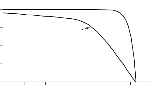
Figure 8.27 Series and parallel resistances in the PV equivalent circuit decrease both

voltage and current delivered. To improve cell performance, high R

and low R

are

needed.

8.4 FROM CELLS TO MODULES TO ARRAYS

Since an individual cell produces only about 0.5 V, it is a rare application for

which just a single cell is of any use. Instead, the basic building block for PV

applications is a module consisting of a number of pre-wired cells in series, all

encased in tough, weather-resistant packages. A typical module has 36 cells in

series and is often designated as a “12-V module” even though it is capable

of delivering much higher voltages than that. Some 12-V modules have only 33

cells, which, as will be seen later may, be desirable in certain very simple battery

charging systems. Large 72-cell modules are now quite common, some of which

have all of the cells wired in series, in which case they are referred to as 24-V

modules. Some 72-cell modules can be ﬁeld-wired to act either as 24-V modules

with all 72 cells in series or as 12-V modules with two parallel strings having

36 series cells in each.

Multiple modules, in turn, can be wired in series to increase voltage and in

parallel to increase current, the product of which is power. An important element

in PV system design is deciding how many modules should be connected in

series and how many in parallel to deliver whatever energy is needed. Such

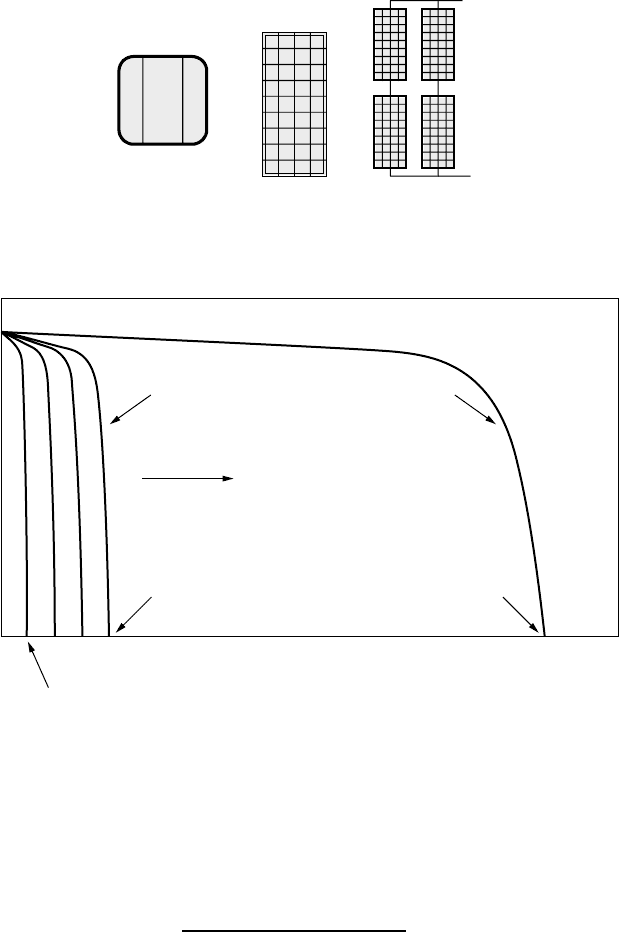
combinations of modules are referred to as an array. Figure 8.28 shows this

distinction between cells, modules, and arrays.

8.4.1 From Cells to a Module

When photovoltaics are wired in series, they all carry the same current, and at

any given current their voltages add as shown in Fig. 8.29. That means we can

continue the spreadsheet solution of (8.18) to ﬁnd an overall module voltage

FROM CELLS TO MODULES TO ARRAYS 469

Cell Module Array

Figure 8.28 Photovoltaic cells, modules, and arrays.

0.6 V for each cell

VOLTAGE (V)

CURRENT (A)

21.6 V

4 cells

Adding cells in series

36 cells

2.4 V

36 cells × 0.6 V = 21.6 V

Figure 8.29 For cells wired in series, their voltages at any given current add. A typical

module will have 36 cells.

module

by multiplying (8.21) by the number of cells in the module n.

module

= n(V

− IR

)(8.22)

Example 8.4 Voltage and Current from a PV Module. A PV module is made

up of 36 identical cells, all wired in series. With 1-sun insolation (1 kW/m

each cell has short-circuit current I

= 3.4Aandat25

◦

C its reverse saturation

current is I

= 6 × 10

−10

A. Parallel resistance R

= 6.6  and series resistance

= 0.005 .

470 PHOTOVOLTAIC MATERIALS AND ELECTRICAL CHARACTERISTICS

a. Find the voltage, current, and power delivered when the junction voltage

of each cell is 0.50 V.

b. Set up a spreadsheet for I and V and present a few lines of output to show

how it works.

Solution.

a. Using V

= 0.50 V in (8.20) along with the other data gives current:

I = I

− I

38.9V

− 1) −

= 3.4 − 6 ×10

−10

38.9×0.50

− 1) −

0.50

6.6

= 3.16 A

Under these conditions, (8.22) gives the voltage produced by the 36-cell

module:

module

= n(V

− IR

) = 36(0.50 − 3.16 × 0.005) = 17.43 V

Power delivered is therefore

P(watts) = V

module

I = 17.43 × 3.16 = 55.0W

b. A spreadsheet might look something like the following:

Number of cells,n = 36

Parallel resistance/cell R

(ohms) = 6.6

Series resistance/cell R

(ohms) = 0.005

Reverse saturation current I

(A) = 6.00E-10

Short-circuit current at 1-sun (A) = 3.4

I =

− I



38.9V

− 1



−

module

n(V

− IR

)

P (watts)

= V

module

0.49 3.21 17.06 54.80

0.50 3.16 17.43 55.02

0.51 3.07 17.81 54.75

0.52 2.96 18.19 53.76

0.53 2.78 18.58 51.65

0.54 2.52 18.99 47.89

0.55 2.14 19.41 41.59

FROM CELLS TO MODULES TO ARRAYS 471

Notice that we have found the maximum power point for this module, which

is at I = 3.16 A, V = 17.43 V, and P = 55 W. This would be described as a

55-W module.

8.4.2 From Modules to Arrays

Modules can be wired in series to increase voltage, and in parallel to increase

current. Arrays are made up of some combination of series and parallel modules

to increase power.

For modules in series, the I –V curves are simply added along the voltage

axis. That is, at any given current (which ﬂows through each of the modules),

the total voltage is just the sum of the individual module voltages as is suggested

in Fig. 8.30.

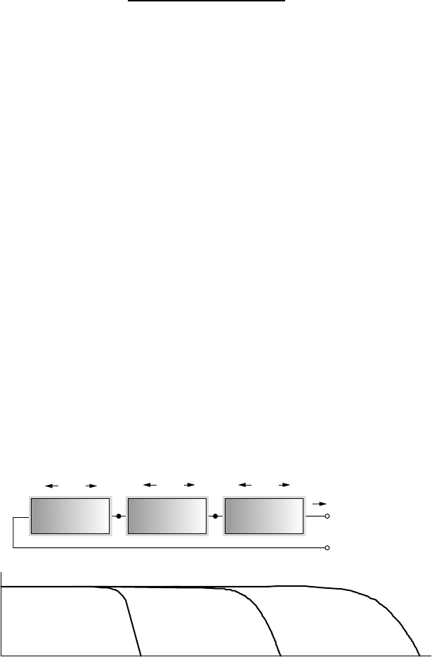
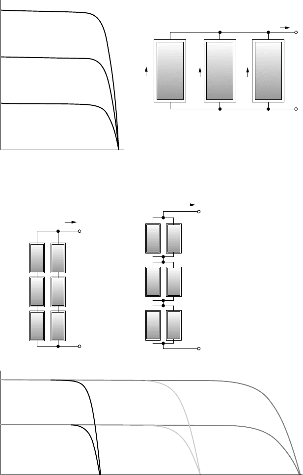
For modules in parallel, the same voltage is across each module and the total

current is the sum of the currents. That is, at any given voltage, the I –V curve

of the parallel combination is just the sum of the individual module currents at

that voltage. Figure 8.31 shows the I –V curve for three modules in parallel.

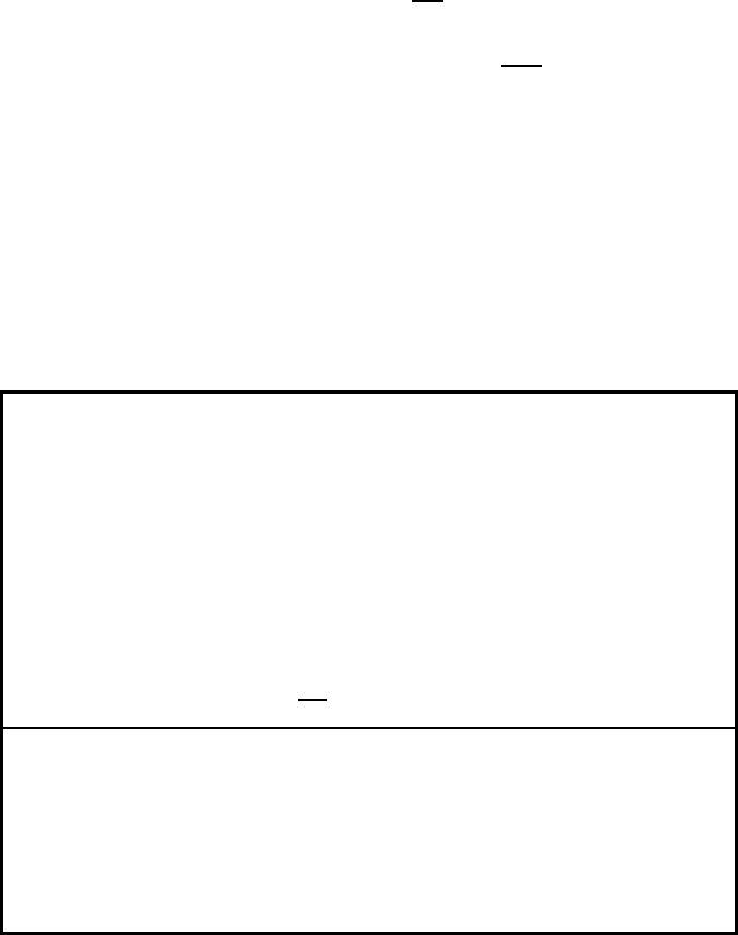
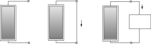
When high power is needed, the array will usually consist of a combination

of series and parallel modules for which the total I –V curve is the sum of

the individual module I –V curves. There are two ways to imagine wiring a

series/parallel combination of modules: The series modules may be wired as

strings, and the strings wired in parallel as in Fig. 8.32a, or the parallel modules

may be wired together ﬁrst and those units combined in series as in 8.32b.

The total I –V curve is just the sum of the individual module curves, which

is the same in either case when everything is working right. There is a reason,

however, to prefer the wiring of strings in parallel (Fig. 8.32a). If an entire string

is removed from service for some reason, the array can still deliver whatever

voltage is needed by the load, though the current is diminished, which is not the

case when a parallel group of modules is removed.

VOLTAGE

CURRENT

1 module 2 modules 3 modules

−

+−

Figure 8.30 For modules in series, at any given current the voltages add.

472 PHOTOVOLTAIC MATERIALS AND ELECTRICAL CHARACTERISTICS

VOLTAGE

CURRENT

1 module

2 modules

3 modules

−

Figure 8.31 For modules in parallel, at any given voltage the currents add.

VOLTAGE

CURRENT

(c)

(a)

(b)

−

Figure 8.32 Two ways to wire an array with three modules in series and two modules in

parallel. Although the I –V curves for arrays are the same, two strings of three modules

each (a) is preferred. The total I –V curve of the array is shown in (c).

THE PV I–V CURVE UNDER STANDARD TEST CONDITIONS (STC) 473

8.5 THE PV I–V CURVE UNDER STANDARD TEST CONDITIONS (STC)

Consider, for the moment, a single PV module that you want to connect to some

sort of a load (Fig. 8.33). The load might be a dc motor driving a pump or it

might be a battery, for example. Before the load is connected, the module sitting

in the sun will produce an open-circuit voltage V

, but no current will ﬂow. If

the terminals of the module are shorted together (which doesn’t hurt the module

at all, by the way), the short-circuit current I

will ﬂow, but the output voltage

will be zero. In both cases, since power is the product of current and voltage, no

power is delivered by the module and no power is received by the load. When the

load is actually connected, some combination of current and voltage will result

and power will be delivered. To ﬁgure out how much power, we have to consider

the I –V characteristic curve of the module as well as the I –V characteristic

curve of the load.

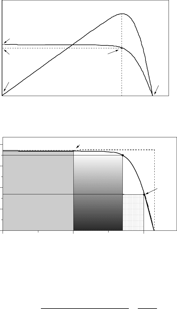
Figure 8.34 shows a generic I –V curve for a PV module, identifying sev-

eral key parameters including the open-circuit voltage V

and the short-circuit

current I

. Also shown is the product of voltage and current, that is, power

delivered by the module. At the two ends of the I –V curve, the output power is

zero since either current or voltage is zero at those points. The maximum power

point (MPP) is that spot near the knee of the I –V curve at which the product of

current and voltage reaches its maximum. The voltage and current at the MPP

are sometimes designated as V

and I

for the general case and designated V

and I

(for rated voltage and rated current ) under the special circumstances that

correspond to idealized test conditions.

Another way to visualize the location of the maximum power point is by

imagining trying to ﬁnd the biggest possible rectangle that will ﬁt beneath the

I –V curve. As shown in Fig. 8.35, the sides of the rectangle correspond to

current and voltage, so its area is power. Another quantity that is often used to

characterize module performance is the ﬁll factor (FF). The ﬁll factor is the ratio

of the power at the maximum power point to the product of V

and I

,so

FF can be visualized as the ratio of two rectangular areas, as is suggested in

(a) (b) (c)

= 0

−

= 0

Open circuit

−

= 0

Short circuit Load connected

LOAD

−

V I

Figure 8.33 No power is delivered when the circuit is open (a) or shorted (b). When

the load is connected (c), the same current ﬂows through the load and module and the

same voltage appears across them.

474 PHOTOVOLTAIC MATERIALS AND ELECTRICAL CHARACTERISTICS

VOLTAGE (V)

POWER ( W)

Power

Current

Maximum Power Point

(MPP)

= 0

CURRENT (A)

Figure 8.34 The I –V curve and power output for a PV module. At the maximum

power point (MPP) the module delivers the most power that it can under the conditions

of sunlight and temperature for which the I –V curve has been drawn.

20100

VOLTAGE (V)

CURRENT (A)

= 70 W

= 120 W

= 74 W

= 7.5 A

= 21.5 V

MPP

Figure 8.35 The maximum power point (MPP) corresponds to the biggest rectangle that

can ﬁt beneath the I –V curve. The ﬁll factor (FF) is the ratio of the area (power) at MPP

to the area formed by a rectangle with sides V

and I

Fig. 8.35. Fill factors around 70–75% for crystalline silicon solar modules are

typical, while for multijunction amorphous-Si modules, it is closer to 50–60%.

Fill factor (FF) =

Power at the maximum power point

(8.23)

IMPACTS OF TEMPERATURE AND INSOLATION ON I–V CURVES 475

TA BLE 8.3 Examples of PV Module Performance Data Under Standard Test

Conditions (1 kW/m

,AM1.5,25

◦

C Cell Temperature)

Manufacturer Kyocera Sharp BP Uni-Solar Shell

Model KC-120-1 NE-Q5E2U 2150S US-64 ST40

Material Multicrystal Polycrystal Monocrystal Triple junction a-Si CIS-thin ﬁlm

Number of cells n 36 72 72 42

Rated Power P

DC,STC

(W)

120 165 150 64 40

Voltage at max

power (V)

16.9 34.6 34 16.5 16.6

Current at rated

power (A)

7.1 4.77 4.45 3.88 2.41

Open-circuit voltage

(V)

21.5 43.1 42.8 23.8 23.3

Short-circuit current

(A)

7.45 5.46 4.75 4.80 2.68

Length (mm/in.) 1425/56.1 1575/62.05 1587/62.5 1366/53.78 1293/50.9

Width (mm/in.) 652/25.7 826/32.44 790/31.1 741/29.18 329/12.9

Depth (mm/in.) 52/2.0 46/1.81 50/1.97 31.8/1.25 54/2.1

Weight (kg/lb) 11.9/26.3 17/37.5 15.4/34 9.2/20.2 14.8/32.6

Module efﬁciency 12.9% 12.7% 12.0% 6.3% 9.4%

Since PV I –V curves shift all around as the amount of insolation changes

and as the temperature of the cells varies, standard test conditions (STC) have

been established to enable fair comparisons of one module to another. Those test

conditions include a solar irradiance of 1 kW/m

(1 sun) with spectral distribution

shown in Fig. 8.10, corresponding to an air mass ratio of 1.5 (AM 1.5). The

standard cell temperature for testing purposes is 25

◦

C (it is important to note that

◦

is cell temperature, not ambient temperature). Manufacturers always provide

performance data under these operating conditions, some examples of which are

shown in Table 8.3. The key parameter for a module is its rated power; to help

us remember that it is dc power measured under standard test conditions, it has

been identiﬁed in Table 8.3 as P

DC,STC

. Later we’ll learn how to adjust rated

power to account for temperature effects as well as see how to adjust it to give

us an estimate of the actual ac power that the module and inverter combination

will deliver.

8.6 IMPACTS OF TEMPERATURE AND INSOLATION ON I–V CURVES

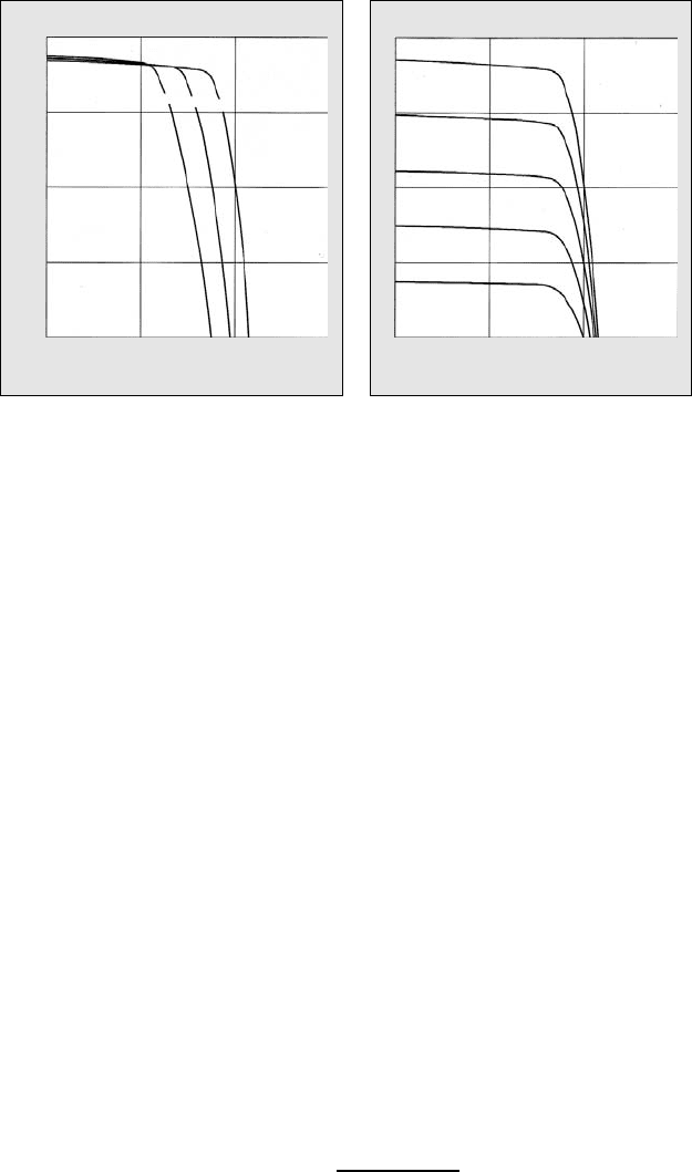
Manufacturers will often provide I –V curves that show how the curves shift

as insolation and cell temperature changes. Figure 8.36 shows examples for the

Kyocera 120-W multicrystal-silicon module described in Table 8.3. Notice as

insolation drops, short-circuit current drops in direct proportion. Cutting insola-

tion in half, for example, drops I

by half. Decreasing insolation also reduces

476 PHOTOVOLTAIC MATERIALS AND ELECTRICAL CHARACTERISTICS

0 102030

0102030

IRRADIANCE: AM1.5, 1 kW/m

Voltage (V) Voltage (V)

Current (A)

1000 W/m

800 W/m

600 W/m

400 W/m

200 W/m

CELL TEMP. 25°C

75°C

50°C

25°C

Figure 8.36 Current-voltage characteristic curves under various cell temperatures and

irradiance levels for the Kyocera KC120-1 PV module.

, but it does so following a logarithmic relationship that results in relatively

modest changes in V

As can be seen in Fig. 8.36, as cell temperature increases, the open-circuit

voltage decreases substantially while the short-circuit current increases only

slightly. Photovoltaics, perhaps surprisingly, therefore perform better on cold,

clear days than hot ones. For crystalline silicon cells, V

drops by about 0.37%

for each degree Celsius increase in temperature and I

increases by approx-

imately 0.05%. The net result when cells heat up is the MPP slides slightly

upward and toward the left with a decrease in maximum power available of

about 0.5%/

◦

C. Given this signiﬁcant shift in performance as cell temperature

changes, it should be quite apparent that temperature needs to be included in any

estimate of module performance.

Cells vary in temperature not only because ambient temperatures change, but

also because insolation on the cells changes. Since only a small fraction of the

insolation hitting a module is converted to electricity and carried away, most of

that incident energy is absorbed and converted to heat. To help system designers

account for changes in cell performance with temperature, manufacturers often

provide an indicator called the NOCT, which stands for nominal operating cell

temperature. The NOCT is cell temperature in a module when ambient is 20

◦

solar irradiation is 0.8 kW/m

, a nd windspeed is 1 m/s. To account for other

ambient conditions, the following expression may be used:

cell

= T

amb



NOCT − 20

◦

0.8



· S(8.24)

SHADING IMPACTS ON I–V CURVES 477

where T

cell

is cell temperature (

◦

C), T

amb

is ambient temperature, and S is solar

insolation (kW/m

Example 8.5 Impact of Cell Temperature on Power for a PV Module.

Estimate cell temperature, open-circuit voltage, and maximum power output for

the 150-W BP2150S module under conditions of 1-sun insolation and ambient

temperature 30

◦

C. The module has a NOCT of 47

◦

Solution. Using (8.24) with S = 1kW/m

, cell temperature is estimated to be

cell

= T

amb



NOCT − 20

◦

0.8



· S = 30 +



47 − 20

0.8



· 1 = 64

◦

From Table 8.3, for this module at the standard temperature of 25

◦

C, V

42.8V.SinceV

drops by 0.37%/

◦

C, the new V

will be about

= 42.8[1 − 0.0037(64 − 25)] = 36.7V

With maximum power expected to drop about 0.5%/

◦

C, this 150-W module at

its maximum power point will deliver

max

= 150 W · [1 − 0.005(64 −25)] = 121 W

which is a rather signiﬁcant drop of 19% from its rated power.

When the NOCT is not given, another approach to estimating cell temperature

is based on the following:

cell

= T

amb

+ γ



Insolation

1kW/m



(8.25)

where γ is a proportionality factor that depends somewhat on windspeed and

how well ventilated the modules are when installed. Typical values of γ range

between 25

◦

C and 35

◦

C; that is, in 1 sun of insolation, cells tend to be 25–35

◦

hotter than their environment.

8.7 SHADING IMPACTS ON I –V CURVES

The output of a PV module can be reduced dramatically when even a small

portion of it is shaded. Unless special efforts are made to compensate for shade

problems, even a single shaded cell in a long string of cells can easily cut