Zhang K., Li D. Electromagnetic Theory for Microwaves and Optoelectronics

Подождите немного. Документ загружается.

4.10 Vector Eigenfunctions and Normal Modes 221

Theorem 2 All eigenvalues are nonnegative for q ≤ 0, and with the con-

stant boundary conditions (4.240),

≥ 0.

Theorem 3. Orthogonality Theorem The eigenfunction set is a com-

plete orthogonal set. The eigenfunctions y

(x) and y

(x) corresponding to

eigenvalues λ

and λ

, respectively, are orthogonal with weight ρ(x).

ρ(x)y

∗

(x)y

(x)dx = 0, m 6= n. (4.241)

Theorem 4. Expansion Theorem Every continuous function f(x) which

has piecewise continuous ﬁrst and second derivatives and satisﬁes the bound-

ary conditions of the eigenvalue problem can be expanded in an absolutely

and uniformly convergent series in terms of the eigenfunctions

f(x) =

∞

n=1

(x). (4.242)

The coeﬃcients a

can be obtained by using the orthogonality property of

the eigenfunctions:

ρ(x

)f(x

∗

)dx

ρ(x

)|y

. (4.243)

The proofs of the above theorems can be found in texts on mathematical

physics, for example [26, 35, 72].

(2) Orthonormal Eigenfunction Set

Deﬁne a set of normalized orthogonal eigenfunctions, namely orthonormal

eigenfunctions as follows:

(x) =

(x)

ρ(x)|y

(x)|

. (4.244)

The orthogonal relation of the orthonormal eigenfunctions becomes

ρ(x)U

∗

(x)U

(x)dx = δ

, δ

0, n 6= m,

1, n = m.

(4.245)

The expansion of the function f(x) in terms of the orthonormal eigenfunctions

(x) is

f(x) =

∞

n=1

(x). (4.246)

222 4. Time-Varying Boundary Value Problems

The coeﬃcients a

become

ρ(x

)f(x

∗

)dx

. (4.247)

(3) Completeness Relation

Substituting the coeﬃcient a

(4.247) into the series (4.246), we have

f(x) =

∞

n=1

ρ(x

)f(x

∗

)dx

(x)

∞

n=1

ρ(x

∗

(x)

f(x

)dx

, (4.248)

where x is a speciﬁc point and x

is the integration variable. The point x lies

within the range a–b, applying the functional property of the δ function,

δ(x

− x)f(x

)dx

= f(x),

we have the completeness relation:

∞

n=1

ρ(x

∗

(x) = δ(x

− x). (4.249)

If ρ(x) = 1, the orthonormality condition and the completeness condition

become

∗

(x)U

(x)dx = δ

∞

n=1

∗

(x) = δ(x

− x), (4.250)

and the coeﬃcient a

of the series (4.246) becomes

f(x

∗

)dx

. (4.251)

4.10.2 Eigenvalues for the Boundary-Value Problems

of the Vector Helmholtz Equations

The general solutions of the Helmholtz’s equations in the commonly used

coordinate systems obtained in the previous sections are the vector eigen-

functions. The eigenvalues of the boundary value problems of the vector

Helmholtz equations are given by

= k

+ k

, for rectangular coordinates, (4.252)

4.10 Vector Eigenfunctions and Normal Modes 223

= β

+ T

with ν or n, for cylindrical coordinates, (4.253)

, with n, m, for spherical coordinates, (4.254)

where k

, k

, T

, ν, n, and m are the eigenvalues of the corresponding

ordinary diﬀerential equations. Each of them is an inﬁnite set of discrete

values. The eigenvalue of the vector Helmholtz equations, k

, is then an

inﬁnite set of discrete values too, denoted by k

Each of the eigenvalues corresponds to a speciﬁc set of vector eigenfunc-

tions E

(x) and H

(x), which is known as a normal mode. The vector

eigenfunctions satisfy the vector Helmholtz equations in a volume V and

given boundary conditions of the ﬁrst or the second kind, including the short-

circuit or the open-circuit boundary conditions on the boundary S enclosing

V .

For source-free problems, ∇ · E

= 0, the vector Helmholtz equation for

(4.21) can be written as

∇ × ∇ × E

− k

= 0. (4.255)

Taking the scalar product of (4.255) with E

∗

, then integrating over V , gives

dV =

∗

· (∇ × ∇ × E

) dV. (4.256)

Applying the vector identity (B.38) for ∇ · (A × B), we have

∗

· (∇ × ∇ × E

) = |∇ × E

− ∇ · (E

∗

× ∇ × E

Substituting this into (4.256) and using the Gauss’ formula yields

dV =

|∇ × E

dV −

∗

× ∇ × E

) · n dS. (4.257)

Applying the triple scalar product formula (B.29), we may write the integrand

of the second term on the right-hand side of (4.257) as

n · (E

∗

× ∇ × E

) = ∇ × E

· (n × E

∗

n · (E

∗

× ∇ × E

) = −E

∗

· (n × ∇ × E

) = E

∗

· j ω ˙µ(n × H

Nevertheless the ﬁelds satisfying the short-circuit boundary condition, ∇ ×

= 0, or the open-circuit boundary condition, ∇ × H

= 0, means

that the second term of the right-hand side of (4.257) is equal to zero, so that

|∇ × E

. (4.258)

224 4. Time-Varying Boundary Value Problems

This is the expression of the eigenvalue of the boundary value problem for

the vector Helmholtz equation.

The integrands in the numerator and the denominator on the right-hand

side of (4.258) cannot be negative. So we have

≥ 0. (4.259)

So k

is a set of inﬁnite discrete real numbers. This is the basic property

of the eigenvalues of the Strum–Liouville problems. The physical meaning of

is the natural angular wave number of the mth mo de in a closed system.

The corresponding natural angular frequency is

√

µ²

, (4.260)

which is also a set of inﬁnite discrete values. In a lossless closed system,

the electromagnetic ﬁelds can exist only when the frequency of the sinu-

soidal ﬁelds equals one of the natural frequencies, and the ﬁeld distribution

is described by the vector eigenfunctions of the corresponding mode. So any

closed system is a resonant system.

4.10.3 Two-Dimensional Eigenvalues in Cylindrical

Systems

If there are no boundaries in the longitudinal direction z, a cylindrical system

becomes a uniform transmission system or guided-wave system. The problem

reduces to a two-dimensional boundary value problem. For a source-free

system, the two-dimensional Helmholtz equation (4.96) becomes

∇

× ∇

× E

+ T

= 0. (4.261)

satisﬁes the short-circuit or open-circuit boundary conditions at the

closed curve l surrounding the cross section S of the system. T

is the

two-dimensional eigenvalue of the problem. Similarly, we have

|∇

× E

. (4.262)

is also a set of inﬁnite discrete positive values, T

≥ 0, and T

is real or

zero. The physical meaning of T

= k

is the cutoﬀ angular wave number

of the mth mode in the transmission system, and the critical or the cutoﬀ

angular frequency is

√

µ²

, (4.263)

The longitudinal phase constant β = k

becomes continuous:

− T

, (4.264)

4.10 Vector Eigenfunctions and Normal Modes 225

and

≤ k, v

= ω/β

≥ 1/

√

µ².

So a uniform cylindrical system enclosed by smooth short-circuit or open-

circuit boundaries is always a fast wave system or a system with a phase

velocity equal to the unbounded speed of light, and can never be a slow wave

system. A slow wave system must be enclosed by a boundary of impedance

surfaces.

4.10.4 Vector Eigenfunctions and Normal Mode

Expansion

The vector eigenfunction set of the time-varying boundary-value problems

forms a complete orthogonal set.

In a cylindrical system, (u

, u

, z), suppose that the two-dimensional vec-

tor eigenfunctions of two arbitrary modes are E

, u

), H

, u

) and

, u

), H

, u

), the transverse two-dimensional eigenvalues are T

and the longitudinal phase constants are β

, β

, respectively. The or-

thogonality of these two sets of vector eigenfunctions is given as

, u

) × H

∗

, u

)] · ˆzdS = 0, n 6= m, (4.265)

where S

denotes an arbitrary cross section of the system. Note that E

, E

, and H

here are functions of the the two-dimensional coordinates

on the cross section (u

, u

). The physical meaning of this expression is that

the electric ﬁeld and magnetic ﬁeld of two diﬀerent modes do not carry any

power ﬂow. So the total power ﬂow of a multi-mode system is equal to the

sum of the power ﬂows of all modes. These modes are known as normal

modes.

According to the Lorentz’s reciprocal theorem in the source-free region

(1.289)

× H

∗

− E

∗

× H

) · ndS = 0, (4.266)

where S is the closed surface surrounding the volume to be investigated.

Note that E

, H

, E

, and H

here are functions of the three-dimensional

coordinates (u

, u

, z) or (x).

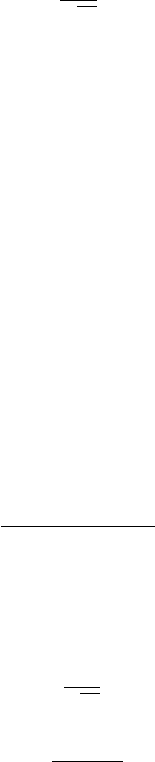
The region to be investigated is a segment of a source-free cylindrical

system. The surface S consists of two parts, i.e., the two arbitrary cross-

section surfaces S

and S

at z

and z

, and the cylindrical surface S

between

and z

, see Fig. 4.8. Then (4.266) becomes

× H

∗

− E

∗

× H

) · ˆzdS −

× H

∗

− E

∗

× H

) · ˆzdS

× H

∗

− E

∗

× H

) · ndS = 0. (4.267)

226 4. Time-Varying Boundary Value Problems

Figure 4.8: A segment of a source-free cylindrical system.

For metallic waveguides, the cylindrical surface S

is the conducting wall,

and for the dielectric waveguide, S

is the cylindrical surface between S

and

at inﬁnity or far enough away so that the ﬁelds vanish. So the tangential

components of the ﬁeld are zero on the cylindrical surface S

, and the third

integral of (4.267) is zero. The equation becomes

×H

∗

−E

∗

×H

)·ˆzdS−

×H

∗

−E

∗

×H

)·ˆzdS = 0. (4.268)

The two cross sections S

and S

are arbitrary chosen. To satisfy the above

equation, we must have

× H

∗

− E

∗

× H

) · ˆzdS = 0, (4.269)

where S

is a cross section at an arbitrary z.

If the two modes are both traveling waves in the +z direction,

(x) = E

, u

−jβ

, H

(x) = H

, u

−jβ

(x) = E

, u

−jβ

, H

(x) = H

, u

−jβ

then (4.269) becomes

−j(β

−β

, u

)×H

∗

, u

)−E

∗

, u

)×H

, u

)] · ˆzdS =0.

For non-degenerate modes, β

6= β

, we have

, u

)×H

∗

, u

)−E

∗

, u

)×H

, u

)] · ˆzdS = 0. (4.270)

If the nth mode is a traveling wave in the +z direction, and the mth mode

is a traveling wave in the −z direction,

(x) = E

, u

−jβ

, H

(x) = H

, u

−jβ

(x) = E

, u

jβ

, H

(x) = −H

, u

jβ

4.10 Vector Eigenfunctions and Normal Modes 227

then (4.269) becomes

−j(β

+β

[−E

, u

)×H

∗

, u

)−E

∗

, u

)×H

, u

)]·ˆzdS = 0,

and we have

[−E

, u

)×H

∗

, u

)−E

∗

, u

)×H

, u

)]·ˆzdS =0. (4.271)

Taking the sum and the diﬀerence of (4.270) and (4.271), gives

∗

, u

) × H

, u

)] · ˆzdS = 0, (4.272)

, u

) × H

∗

, u

)] · ˆzdS = 0. (4.273)

The orthogonality of normal modes is proven.

Any ﬁelds over the cross section of a cylindrical system can thus be ex-

panded into a series of vector eigenfunctions or normal modes:

E =

∞

n=1

, H =

∞

n=1

. (4.274)

The coeﬃcients of the series may be obtained by the orthogonality principle:

(E × H

∗

) · ˆzdS

× H

∗

) · ˆzdS

, B

∗

× H) · ˆzdS

∗

× H

) · ˆzdS

. (4.275)

Deﬁne the orthonormal vector eigenfunctions as

× H

∗

) · ˆzdS

, h

∗

× H

) · ˆzdS

. (4.276)

Then the orthonormal mode expansions of the ﬁelds become

E =

∞

n=1

, H =

∞

n=1

, (4.277)

and the coeﬃcients become

(E × h

∗

) · ˆzdS, b

∗

× H) · ˆzdS. (4.278)

We come to the conclusion that the solutions of the Helmholtz’s equations

that satisfy speciﬁc boundary conditions is a complete set of inﬁnite number

of normal modes. A ﬁnite number of modes are propagation modes or guided

modes and the rests are cutoﬀ modes or evanescent modes.

The orthogonality of the three-dimensional vector eigenfunctions can also

be proven and any ﬁelds in a closed region can also be expanded into a series

of the three-dimensional orthonormal vector eigenfunctions. [91]

228 4. Time-Varying Boundary Value Problems

4.11 Approximate Solution of

Helmholtz’s Equations

If the boundaries of the region coincide with the surfaces of a coordinate

system and are uniform along the three axes, the problem is known as a

simple boundary problem. Otherwise, it is a complicated boundary problem.

The exact solution of a simple boundary problem can be easily obtained

by means of separation of variables. For the complicated boundary problem,

the exact solution is usually diﬃcult to obtain, and we have to ﬁnd the

approximate solution under certain conditions. The approximate solution

includes approximate eigenvalues and approximate eigenfunctions.

4.11.1 Variational Principle of Eigenvalues

Suppose E is a ﬁeld satisfying Helmoltz’s equation,

∇ × ∇ × E − k

E = 0, (4.279)

but not totally satisfying the boundary conditions.

Taking the scalar product of (4.279) with E

∗

, and integrating over V , we

have

E · E

∗

dV =

∗

· ∇ × ∇ × E dV, (4.280)

which gives

∗

· ∇ × ∇ × E dV

E · E

∗

= X(E). (4.281)

This shows that the eigenvalue k

is a functional in terms of the vector

function E. When the boundary conditions are totally satisﬁed, E becomes

the true eigenfunction or true ﬁeld and k

becomes the true eigenvalue of the

problem shown in (4.258).

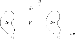
We are now going to show the stationary character of the eigenvalue k

Supposing E is the true ﬁeld, and E

is the approximate solution, which is

called trial function and δE denotes the deviation between E

and E:

= E + δE. (4.282)

Taking the variation of (4.280), we have

E · E

∗

= δ

∗

· ∇ × ∇ × E dV

. (4.283)

Note that the regulations of the variation of a functional are similar to those

of the diﬀerentiation of a function. Then the variational equation (4.283)

4.11 Approximate Solution of Helmholtz’s Equations 229

Figure 4.9: Stationary formula (a), and non-stationary formula (b).

becomes

E · E

∗

δk

δE

∗

∇ × ∇ × E − k

∗

∇ × ∇ × δE − k

δE

dV. (4.284)

The ﬁrst term on the right-hand side of the above equation must be zero,

because the true ﬁeld satisﬁes Helmholtz’s equation (4.279). Suppose that

the trial ﬁeld E

also satisﬁes Helmholtz’s equation, then the second term is

also zero

∇ × ∇ × δE − k

δE = 0.

The integral on the left-hand side,

E ·E

∗

dV =

dV , cannot be zero,

so we have

δk

= 0. (4.285)

The ﬁrst-order variation of the functional k

is equal to zero at δE = 0. This

means that k

will have a minimum or maximum at δE = 0, and the formula

(4.281) is known as the stationary formula of the eigenvalue k

. See Fig. 4.9.

It is evident that for small δE the stationary formula gives a smaller error

in k

than does the non-stationary formula. This property is summarized as

follows: A parameter determined by a stationary formula is insensitive to

small variations of the ﬁeld about the true ﬁeld. In this case the error in

the parameter is smaller then that in the ﬁeld in one order. An error of the

order of 10% in the trial ﬁeld E

gives an error of the order of only 1% in

the eigenvalue k

when the trial ﬁeld satisﬁes Helmholtz’s equation but does

not totally satisfy the boundary conditions.

A stationary formula for the trial ﬁeld, which satisﬁes the boundary con-

ditions but does not satisfy Helmholtz’s equation, can also be derived [37].

The two-dimensional eigenvalue T

in the cylindrical system is given by

∗

· ∇

× ∇

× E dS

E · E

∗

= X(E), (4.286)

230 4. Time-Varying Boundary Value Problems

which is also a stationary formula, and

δT

= 0. (4.287)

In the analysis of the resonant system or transmission system, the value

of the nature frequency, which is determined by k

, or the cutoﬀ frequency,

which is determined by T

, must be more accurate than the distribution of

the ﬁelds. This requirement is consistent with the variational principle of the

eigenvalues.

4.11.2 Approximate Field-Matching Conditions

For some problems with complicated boundaries, the whole region can be di-

vided into a number of subregions, and the problem becomes a simple bound-

ary condition problem in each subregion. The uniqueness theorem of such

problems is given in Section 4.1.2. The appropriate boundary conditions, or

so called ﬁeld matching conditions, over the boundaries for the accurate so-

lution are given in (4.5). Sometimes the exact ﬁeld expressions and the exact

equation for the eigenvalues, which is known as the characteristic equation,

are extremely complicated. So we want to ﬁnd out the approximate boundary

conditions for the best approximate solution.

Consider a complicated region of volume V enclosed by a short-circuit or

open-circuit boundary S. The whole region is divided into n subregions with

simple boundaries V

, i = 1 to n. The subregion V

is enclosed by S

, which

consists of two sorts of surfaces, the outer boundary of the whole region V

denoted by S

, which is a part of S, and the inner boundary or interface

between subregion V

and the adjacent subregion V

, denoted by S

. See

Fig. 4.1b.

According to the uniqueness theorem given in Section 4.1.2, the true ﬁelds

(x), H

(x) must satisfy the following Helmholtz equations and boundary

conditions on the outer boundaries S

as well as the matching conditions on

the inner boundaries S

∇ × ∇ × E

− k

= 0, ∇ × ∇ × H

− k

= 0,

n × E

= 0 or n × H

= 0,

n × E

= n × E

and n × H

= n × H

According to the variational principle given in the above subsection, we

can ﬁnd a set of approximate solutions as the trial ﬁelds E

(x), H

(x),

which satisfy Helmholtz’s equations and the boundary conditions on the outer

boundaries,

∇ × ∇ × E

− k

= 0, (4.288)

∇ × ∇ × H

− k

= 0, (4.289)

n × E

= 0 or n × H

= 0. (4.290)